>> (75.00 + 89.50 + 97.50) / 3 * 0.7 + 92.00 * 0.3
    88.73333333
The expression may contain numbers and
operators +, -, *, and / that represent addition, subtraction, multiplication,
and division, and parentheses can be used for grouping.
| + | addition |
| - | subtraction |
| * | multiplication |
| / | division |
| ^ | a^b is equal to |
| () | grouping |
Finding the square root of ![]()
>> (6^2 + 8^2)^(1/2)
    10
Numbers can also be enter using exponential format. For example,
-1.1e-3 is the same as -0.0011, and 1e+6 or
1e6 is another way of writing 1000000, a million.
>> sqrt(6^2 + 8^2)
    10
The built-in name for exponential function
>> cos(pi)
    -1
>> sin( pi)
   1.224606354e-16
Note that the exact answer to
>> sqrt(3M)
   1.73205080756887729352744634150587E0
>> x = 3.14159265358979323846264338327950M
     3.14159265358979323846264338327950E0
>> sqrt(x)
     1.77245385090551602729816748334114E0
The precision of MPF can be rest by assigning a multiple to global variable
global.mpf_ndigits.
The default value of mpf_ndigits is 128, therefore an mpf may have 128 significant binary digits as opposed to 52 for double. The value of mpf_ndigits. can be set to a multiple (at least 2) of 32.
If a number has the suffix L it is treated as a long integer, which can be as big as the computer memory allows. For example
>> 128L ^ 20L
     1393796574908163946345982392040522594123776
>> sqrt(-5)
    0 + 2.236067977i
>> (3+5i) / (2-3j)
    -0.6923076923 + 1.461538462i
>> h = 1.25creates a variable named ``h'' and assign value 1.25 to it. If there is already a variable named ``h'', then its value will be updated to 1.25.
The interpreter remembers the values of the variables, so that you can recall the names of the variables to use their values. For example:
>> c = 10;
>> b = 8;
>> sqrt(c^2 - b^2)
    6
A variable name can be a string of letters and digits, and underscore _, but cannot begin with a digit. For example, x1, value_1, and _val03 are all valid variable names.
>> h = 1.25
   1.25
To prevent this, a semicolon can be appended. By suppressing unwanted displays, the command window can be kept cleaner and the program may run more efficiently.
>> h = 1.25;
>> // nothing is displayed here
You can always type the commands directly in the command window and see the answers right away.
Alternatively, you can edit all the commands using a text editor and when you are done, copy the commands to clipboard and then paste it to the Shang interpreter window. This can be more efficient since whenever anything goes wrong, you just need to correct the commands in the text editor and paste them again and don't have to retype everything.
When you press enter, if the interpreter doesn't show answer, but keep opening new lines, it thinks the input commands are not complete. It is expecting some closing brackets or quotes. If you want to start over and abondon the current commands, use the ctrl-a command.
 f = (h, r, theta) -> r^2 + h * (1 + cos(theta));
 h = 3.5;
 r = 5;
 theta = pi / 2;
 f(h, r, theta)
In the interactive mode, if the following command is issued
>> run("testscript.txt");
   28.5
>>
All the commands in the script file will be executed.
>> // this is a comment
>> sqrt(-3)   // this is a comment as well
>> /* this is a comment
      this is still a comment
		this is  still a comment
      ...
      we're done commenting (finally) */
Shang interpreter can recognize five levels of nested comments.
if f(a) * f(c) < 0
       b = c;
end
If we want to assign c to b when the condition f(a) * f(c) < 0 is true, and assign c to a when the condition is false:
if f(a) * f(c) < 0
       b = c;
else
       a = c;
end
To test the condition ``n equals to 1'', we need to use two equal signs, like n == 1, not n = 1. Note that a single = is the assignment operator. The statement n = 1 would assign 1 to n instead of testing the condition. The following assigns c to b when n equals 1, and assigns c to a when n equals to 2:
if n == 1
       b = c;
elseif n == 2
       a = c;
end
s = 0;  // initialize s
for k = 1 : 1000000
    s += k;      // add k to s --- equivalent to "s = s + k"
end
The above loop compute the sum

s = 0;
k = 1;
while k <= 1000000   // do the following as long k is less than a million
    if k % 2 != 0    // k % 2 is the remainder of k/2
       s += k;
    end
    ++k;   // increment k, same as k = k + 1;
           // without the increment, k will stays as 1 and loop runs forever
end
The above while loop sums up all the odd numbers between 1 and a
million; it is equivalent to the following for loop
s = 0;
for k = 1 : 2 : 1000000
    s += k;
end
A loop can be stopped by using break statement. For example
f = fopen("shopping-list.txt", "r");
while 1
    line = f.readline();   // read line from the file
    if line == ()          // line is empty --- file end reached
         break;
    end
    // process each line of the file
    // ...
end
Note that since the logical value of 1 is true, while 1
starts an infinite loop (so it has to be stopped by a break somewhere).
Besides for ... end and while ... end loops, in the Shang reference manual you can also find details about the following different types of loops
   until ... end
   do ... while
   do ... until
f = x -> (1 - x) / (1 + x + x^2)A defined function can be called in the obvious way
f = x -> (1 - x) / (1 + x + x^2)  // define a function
f(-1)  // call the function
A function can have several input arguments. For example
f = (r, theta) -> r * (1 + cos(theta)); // define
function_name = function (input_arguments) -> (output arguments)
                    ... // a bunch of statements
                end
Note that in the body of the function, the input arguments can be used as if
they are variables (but they are not visible outside the function), and the
output arguments should be given values before the end of the function.
The following function evaluates the Taylor expansion of
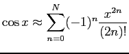
cos_taylor = function (x, N) -> v
       v = 1;
       vk = 1;
       xsq = x * x;
       for k = 1 : N
           vk = - vk * xsq / (2 * k) / (2 * k - 1);
           v += vk;
       end
end
>> A = [1,4, 9; 2, 3, 5; -2, 5, 10]
   1   4    9
   2   3    5
  -2   5   10
To refer to the element of matrix A at second row and third column, use A[2,3]
>> A[2,3]
   5
Create Matrices
Alternatively, a matrix of a required size can be created and initialized using built-in functions zeros, ones, or rand. The command
A = zeros(3, 5)will return a matrix of three rows and five columns, with each element being zero. Similar usage of ones and rand will create matrices of 1's and random numbers (between 0 and 1) respectively.
These three functions can also be called with a single parameter, in which case the second parameter is assumed to be 1, and thus a column vector is created.
>> B = rand(5)
    0.289
    0.353
    0.154
    0.566
    0.821
By the dimension of a matrix we refer to the number of rows
and the number of columns. For example, the dimension of the scalar -5 is
   -2    3    9
    10   1    -2
is
Create Even Spaced Vectors Using the Colon Operator
The symbol : can be used to create a row matrix whose elements are evenly spaced. The default step-size of the vector is 1, which is assumed when one colon is used.
>> A = -1 : 5
   -1  0  1  2  3   4   5
To specify a step-size other than 1, two colons are needed.
>> A = 3 : 0.5 : 5
   3  3.5  4  4.5  5
When you use A : B to create a vector, the value B is not always included in the vector. Alternatively, the built-in function linspace can be used to created even spaced vector with the specified end points included. linspacea, b, n will create a column vector of length n, with a and b being the two end points.
>>  A = [3, 5, -2, 7, 0.9];
>>  A[3]
    -2
The index itself can be vector such that a bunch of the elements of A
are referenced.
>>  A = [3, 5, -2, 7, 0.9];
>>  A[[1, 3, 5]]
    3  -2   0.9
>> A[1:3]
    3   5    -2
>> A[1 : 2 : 5]   // 1 : 2 : 5 is the same as [1, 3, 5]
    3  -2   0.9
The dollar sign $ when used as an index, is the largest value of the
index, therefore A[$] is the last element of A.
>>  A = [3, 5, -2, 7, 0.9];
>>  A[$]
    0.9
>>  A[3:$]
    -2  7  0.9
If matrix A is not a vector, then the element referred to by A[k] is the k-th element of the row vector obtained by horizontally joining all the rows of A.
>> A = [1,4, 9; 2, 3, 5; -2, 5, 10]
   1   4    9
   2   3    5
  -2   5   10
>> A[5]
   3
>> A[9]
   10
>> A = [8, 1, 6; 3, 5, 7; 4, 9, 2]
   8    1    6
   3    5    7
   4    9    2
>> A[2,3]
   7
>> A[1, 1 : 3]   // the first row
   8    1    6
>> A[1 : 3, 2]   // the second column
   1
   5
   9
>> A[[2, 3], [2, 3]]  // the 2x2 submatrix on the lower right corner
   5    7
   9    2
>> A = [8, 1, 6; 3, 5, 7; 4, 9, 2]
   8    1    6
   3    5    7
   4    9    2
>> A[1, :]   // the first row
   8    1    6
>> A[:, 2]   // the second column
   1
   5
   9
>> A[1 : 2, :]  // the first two rows
   8    1    6
   3    5    7
>> A = [8, 1, 6; 3, 5, 7; 4, 9, 2]
   8    1    6
   3    5    7
   4    9    2
>> A[1, :]   // the first row
   8    1    6
>> A[:, 2]   // the second column
   1
   5
   9
>> A[1 : 2, :]  // the first two rows
   8    1    6
   3    5    7
>> A = zeros(3,5)
   0   0   0   0   0
   0   0   0   0   0
>> A[2,3]=2.3
   0   0    0    0   0
   0   0  2.3    0   0
>> A[:, 1] = [5; 10]
    5   0    0    0   0
   10   0  2.3    0   0
>> A[:, 3] = A[:, 3}  + A[:, 1]
    5   0     5    0   0
   10   0  12.3    0   0
>> A[2, :] = 9
    5   0     5    0   0
    9   9     9    9   9
Usually when an indexing expression is used as an lvalue, the dimension and size of the
right hand side of the assignment should match that of the indexing expression to make
the assignment possible. The only exception is when the right hand side is a scalar, then
all the indexed elements of the matrix will be set to the same value.
>> A = zeros(3,3)
   0   0   0
   0   0   0
   0   0   0
>> A[\] = 1;
   1   0   0
   0   1   0
   0   0   1
When updating the contents of a matrix, the indices don't have to be within the upper bounds, which makes it possible to make the size of the matrix grow. As the size of a matrix is being extended, the new entries are set to zero, except for those being specified by the assignment statement. For example,
>> X = [1,4,9]
   1   4   9
>> X[4] = 16
   1   4   9   16
>> x[8]=36
   1   4   9    16    0    0   0   36
A+B, A-B are possible only when A and B have the same dimensions, or one of them is a scalar.
A*B is possible only when the number of columns of A equals the number of rows of B, or one of them is a scalar.
>>  A = [1, 2, -3; 2, 1, 5; 0, -1, 5];
>>  b = [3; 1; -2];
>>  x = A \ b
     0.75
     0.75
    -0.25

>>  A * x - b
    0
    0
    0
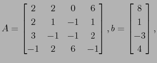
>> A = [2, 2, 0, 6; 2, 1, -1, 1; 3, -1, -1, 2; -1, 2, 6, -1];
>> b = [8; 1; -3; 4];
>> x = A \ b
   -1
    2
    0
    1
>> // verify x is the solution
>> A * x - b
   0
   0
   0
   0
>> norm(A * x - b)
   0
The solution obtained by A
If A is not a square matrix, and b has the same number
of rows as A, then A
b gives the least square solution
to ![]() .
.
To create a polynomial
![]() , do
, do
p = poly[[1, -2, 5, -0.2]];or make a copy of poly and then modify the coeff attribute
p = poly;
p.coeff = [1, -2, 5, -0.2];
If p is a polynomial, p(x) gives the value. Here x can be a scalar, vector, or matrix.
To find the polynomial interpolation through a set of points, do
p = interp(x, y)The result is a polynomial of Newton form and can be called directly.
To create a spline, use splinefit function. For example
>> x = [-1, 0, 1];
>> y = [1.5, 0, 2.5];
>> s = splinefit(x, y);
>> s(x)
    1.5
    0
    2.5
As the result shows, the spline s can be called directly.
s.coeff and s.xnodes give the
coefficient matrix and the nodes of the spline.
Note that the following examples give natural spline, periodic spline,
not-a-knot spline, and clampled spline respectively
   s = splinefit(x, y);
   s = splinefit(x, y, "cyclic");
   s = splinefit(x, y, "not-a-knot");
   s = splinefit(x, y, ypl, ypr);
   // ypl and ypr are the specified derivative values
   //at the left and right end points
One dimensional integral:
int(f, a, b)
Multi-dimensional integral: f has to be a function of one variable, e.g.,
f = x -> exp(-(x[1]^2 + x[2]^2);

int(f, [0, 0], [1, 2])
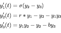
You need to have an ODE function, which takes t and y as input arguments and returns the derivative dy/dt as output values, e.g.,
lorenz = function [sigma = 10, b=8/3, r=28] (t, y) -> yp
                      d1 = sigma * (y[2] - y[1]);
                      d2 = r*y[1] - y[2] - y[1] * y[3];
                      d3 = y[1] * y[2] - b * y[3];
                      yp = [d1; d2; d3];
         end;

// solve the ivp on t=[0, 1]
(t, y) = dsolve(lorenz, [0, 1], [8; 9; 10]);
t is the vector of time values, and y is the matrix whose each
column is the
numerical solution at the corresponding t value.
The complete signature of the dsolve program is
dsolve(ode, tspan, yini, reltol, abstol, ode_type, output_type)
To specify the relative tolerance (default value is ![]() ) as
) as ![]()
(t, y) = dsolve(lorenz, [0, 1], [8; 9; 10], 1e-7);To specify both the relative and the absolute tolerances
(t, y) = dsolve(lorenz, [0, 1], [8; 9; 10], 1e-7, 1e-9);If you know the IVP is stiff or non-stiff problem, you can specify the type as "stiff" or "nonstiff". The default value is "auto".
(t, y) = dsolve(lorenz, [0, 1], [8; 9; 10], 1e-7, 1e-9, "nonstiff");
By default, the solver will output all the time steps and the ![]() values at
these steps. You may require the solver by specifying the final option to report only the
values at
these steps. You may require the solver by specifying the final option to report only the ![]() value at the
final
value at the
final ![]() point, or just return a function (which is an Hermite polynomial
interpolation of the discrete solution). The last option can have values
"recording" (the default), "final", or "interp".
point, or just return a function (which is an Hermite polynomial
interpolation of the discrete solution). The last option can have values
"recording" (the default), "final", or "interp".
(t, y) = dsolve(lorenz, [0, 1], [8; 9; 10], 1e-7, 1e-9, "nonstiff", "final");or
y = dsolve(lorenz, [0, 1], [8; 9; 10], 1e-7, 1e-9, "nonstiff", "interp");
A distribution is a function which when called return random numbers. The built-in distributions include: rand,randz, normal, gauss, gammarv, betarv, binomal, chi, exprv,poisson, frv, student, hypergeom, and multinomial.
Each function is a random number generator. For example, normal(3) returns 3 random numbers of normal distribution. The normal function has two public parameters mu and sigma. To create a new normal distribution, you can reset the parameter values
rv = normal;
rv.mu = 100;
rv.sigma = 15;
The normal function also has common parameters mean,stddev,variance,pdf, cdf, prob, quantile. If you want to calculate the probability that a random variable of distribution rv is between 70 and 130, do
>> rv.prob(70, 130)
   0.9544997361
http://pages.cs.wisc.edu/~ghost/
To use this package, you need to run the file plot.x, which is located in the programs directory. Or just run the following command before you plot
include("plot.x");
The package plot.x defines a class named figure. To make a
plot, first create a figure object using
fig = figure.new();If X and Y are the coordinates of a sequence of points, then
fig.plot(X, Y);will plot Y against X. The result is the points joined by straight line segments.
To plot (X,Y) as dots, use
fig.plot(x=X, y=Y, linetype = "dot");To plot (X,Y) as circles, use
fig.plot(x=X, y=Y, linetype = "circle");To plot a smooth curve through the (x,y) points, use
fig.plot(x=X, y=Y, linetype = "curve");To plot a smooth curve through the (x,y) points, using red color, and making the line thicker
fig.plot(x=X, y=Y, linetype = "curve", linewidth = 2, color=[1,0,0]);When the plotting is done, pick a file name (extension eps) and save the picture
fig.save("file_name.eps");
For example, the following commands will plot some curves and dots
     with("plot.x");
     x = linspace(-5, 5, 10);
     fig = figure.new();
     /* draw small circles at (x,y) locations */
     /* color is vector of 3 numbers between 0 and 1, in rgb format */
     fig.plot{x=x, y=cos(x), linetype="circle", color=[1, 0, 0]};
     /* connect the dots with solid lines, linetype is the default value "solid" */
     fig.plot{x=x, y=cos(x), color=[0,1,0.5]};
     /* draw circular dots at location underneath the previous curve */
     fig.plot{x=x, y=cos(x) -1, linetype="dot", color=[1, 0, 1]};
     /* connect the dots with smooth curve */
     fig.plot{x=x, y=cos(x) -1, linetype="curve", color = [0, 0, 1]};
     /* set the xrange and yrange of the picutre */
     fig.setXrange([-5.5, 5.5]);
     fig.setYrange([-2.5, 1.5]);
     fig.save("curves.eps");
with("plot.x");
fig = figure.new();
for k = 0 : 99
   theta = linspace(k * 2 * pi, (k + 1) * 2 * pi, 500);
   rho = exp(cos(theta)) - 2 * cos(4*theta)+sin(theta/12).^5;
   x = rho .* cos(theta);
   y = rho .* sin(theta);
   fig.plot{x=x, y=y, linetype="curve", color=rand(3)};
end
fig.style = "empty";
fig.save("butterfly.eps");
For more examples, check out Shang website.
f = fopen("Ragu.txt", "r");
Here the file is supposed to located in the current directory. If it's not, the
file name can be an absolute path, or you can use pwd and cd
to change the current working directory.
To read a line of text from an opened fle f.
line = f.readline();The return value line is a character string. When all the lines have been read, f.readline() will return empty list ().
To open a file for writing
fo = fopen("Ragu.txt", "w");
To write a string to file fo
fo.write("abcde");
f.writeline(str) will write a line and append a new newline.
f.printf(format, ...) will print to the file according to a format.
After all operations are done, the file should be closed using
f.close().
Example: the following makes a copy of a file.
f1 = fopen("Ragu.txt", "r");
f2 = fopen("Ragu-1.txt", "w");
if f1 && f2
     line = f1.readline();
     while line != null
          f2.writeline(line);
          line = f1.readline();
     end
end
f1.close();
f2.close();
>> s = "Jerry Gallo."
   Jerry Gallo
You can extract a character or a substring by using operator [] as if it were a vector of characters. For example
>> s = "Jerry Gallo"
   Jerry Gallo
>> s[7]
      G
>> s[7 : 11]
      Gallo
>> s[7] = "C"
   Jerry Callo
Strings can be added
>> s = "The fair breeze blew, " + "the white foam flew."
     The fair breeze blew, the white foam flew.
r = ~/zz*/A regular expression can be used as a function or a set. For example
>> r = ~/zz*/;
>> s = "Jazz";
>> r(s)
   3 4
>> s in r
   1
If the regular expression doesn't match the string, the return value is an empty matrix, otherwise, the starting and ending indices of the match are returned. Or you can use the regular expression as a set. s in r returns either true or false.
>> r = ~s/mate/dude/g;
>> text = "Hey mate, you ...;
>> r(text)
   "Hey dude, you ...?"
Note that the g at the end of the expression stands for ``global``, meaning substituting every occurence of the match. Without the g option, only the first occurence is substituted.
If you want to substutute ``mate`` with "dude" and "Mate" with "Dude", you can do it twice, like
>> r1 = ~s/mate/dude/g;
>> r1 = ~s/Mate/Dude/g;
>> text = r2(r1(text))
Regular expressions can be complicated and powerful. Now suppose that you want to replace every occurence of \code{some text} with
>> r = ~s/\\code{(.*?)}/<font face="Courier New">\1<\/font>/g;
>> text = r(text)
mylist = ("fishhook", "gum", "earplug", "lighter");
To access an element of a list, use the operator #, for example
>> mylist = ("fishhook", "gum", "earplug", "lighter");
>> mylist # 3
   earplug
The index can be vector also
>> mylist = ("fishhook", "gum", "earplug", "lighter");
>> mylist # [2, 3]
   (gum, earplug)
Modify or add an element
>> mylist # 2 = "slingshot";
   (fishhook, slingshot, earplug, lighter);
The length of a list s can be checked by the expression #s.
A list entered this way has a fixed length, meaning you cannot add new elements. For example
>> mylist = ("fishhook", "gum", "earplug", "lighter");
>> mylist # 5 = "tobacco";
   Error: index value 5 out of bound 1-3
If you want the length of the list extendable, you need to append a tilde at the
end of the list
>> mylist = ("fishhook", "gum", "earplug", "lighter");
>> mylist # 6 = "glue";
   (
      fishhook
      gum
      earplug
      lighter
      []
      glue
   )
Note that the fifth element of the list was not given a value, so it got an
empty matrix.
A hash table is another type of collective data. Like list, it contains a collection of values, but each value is not referenced by an index but by a key. For example
anagrams = {"mother in law"       => "woman Hitler",
            "domitory"            => "dirt room",
            "desperation"         => "a rope ends it",
            "election results"    => "lies, let's recount"}
Each element of the table can be extracted and reset
using the operator @.
>> anagrams @ "election results"
   lies, let's recount
>> anagrams @ "astronomer" = "moon starer";
Note that a hash table can have a default key and associated value, whenever k is not a key of the table, t@k returns the value associated with default. For example
>> anagrams @ "default" = "blah";
>> anagrams @ "punishment"
   blah.
A class is a custom defined data type. For example, you want to define a circle class so that all the interested information and attributes of a circle is stored in a variable as a member of the circle class. Suppose that you want to store the center location and the radius of the circle, then you need to specify two attributes. You can define the class like this
circle = class
             public center = [0, 0];
             public radius = 1;
         end;
Here public is the access control type of attribute center,
meaning it can be access inside and outside the class. The two values
[0, 0] and 1 are the default values of the two attributes.
Now, to create a new member of the class
c = circle.new();c will be a member of the class circle and we can check the values of attributes and also reset them
>> c.center
   0  0
>> c. radius
   1
>> c.radius = 10;
>> c.radius
   10
Then function new is the constructor of the class. Note that we didn't write a constructor so the sysem automatically generates a default constructor for us, which assigns the default value to each attribute. If we want to write the constructor by ourself, it's very simple. Just write a function named new which has no output value. The new function returns a class member, whose each attribute obtains the value of the local variable of the new function that has the same name. Any attribute not mentioned in the constructor gets the default value. For example
>> circle = class
             public center = [0, 0];
             public radius = 1;
             new = function (a, b) - ()
                      center = a;
                      radius = b;
                   end
         end;
>> c = circle.new([2, 3], 15);
>> c.center
   2   3
>> c.radius
   15
Note that the constructor new should have no access control type like
public, since it is not a member attribute.
A member attribute can be a function also. Suppose we want to use c.area() and c.perimeter() to find the area and perimeter of the circle, we can do it like this
circle = class
             public center = [0, 0];
             public radius = 1;
             common area = () -> pi * (parent.radius)^2;
         end;
Here common is another access control type. A common attribute
has to be a function and is going to be shared by all members of the class, can
be called but cannot be modified. Inside the attribute function area,
to refer to another attribute of the class member, the keyword parent
has to be used (meaning the class member owns the attribute function being
defined). Here's how to use it
>> circle = class
             public center = [0, 0];
             public radius = 10;
             common area = () -> pi * (parent.radius)^2;
             common perimeter = () -> 2 * pi * (parent.radius);
         end;
>> c = circle.new();
>> c.area()
   314.1592654
>> c.perimeter()
   62.83185307
If c is a member of circle class, c.radius gives the value of the radius attribute and c.radius = -2 modifies the attribute. This is possible due to the fact that radius is a public attribute. A public attribute is accessible and modifiable inside and outside the class. If you don't want to expose an attribute to the outside intrusion and tampering, you can declare it as a private attribute
>> circle = class
             public center = [0, 0];
             private radius = 10;
             common area = () -> pi * (parent.radius)^2;
             common perimeter = () -> 2 * pi * (parent.radius);
         end;
>> c = circle.new();
>> c.area()
   314.1592654
>> c.radius
   Error "c.radius": accessing private attribute 'radius' disallowed
>> c.radius = 25
   Error "c.radius=25":  trying to reset non-public field 'radius'
See, now the radius attribute is hidden and cannot be reset outside the
class.
However, it can be modified internally. For this purpose, we need to write an
attribute function
>> circle = class
             private radius = 10;
             common get_radius = () -> parent.radius;

             common set_radius = function r -> res
                       if r in (0+ to inf)
                          parent.radius = r;
                          res = 1;
                       else
                          res = 0;
                       end
                    end
             common area = () -> pi * (parent.radius)^2;
             common perimeter = () -> 2 * pi * (parent.radius);
         end;
>> c = circle.new();
>> c.set_radius(25);
>> c.get_radius
   25
If you want to write c.area instead of c.area() to get the
area, you can declare the access control type of area to be
auto instead of common
>> circle = class
             private radius = 10;
             auto area = () -> pi * (parent.radius)^2;
         end;
>> c = circle.new();
>> c.area
   314.1592654
An auto attribute has to be a function that takes no input argument.
The only advantage it has over common is calling it doesn't need
().
If you don't want to use get_radius and set_radius, but still want to prevent radius from receiving an invalid value like a negative number, you can use a domain
>> circle = class
             public radius = 10 in (0+ to inf);
             common area = () -> pi * (parent.radius)^2;
             common perimeter = () -> 2 * pi * (parent.radius);
         end;
>> c = circle.new();
>> c.radius
   10
>> c.radius = -5;
   Error "c.radius=-5":  reseting public field 'radius', value out of domain
>> c.radius = 5
   5
Here the domain of radius is 0+ to inf, the interval
A set is a non-ordered collection of values. If x is a member of set s, the expression
x in sevaluates to 1 (true), otherwise, the test value is 0.
There are several ways to implement a set. The first is finite set. Just list all the members of the set and put them in a pair of curly braces, like
>> s = {"Morse", pi, e, [3, 5], 7z};
>> 7z in s
   1
>> "Barber" in s
   0
You can also use the finite set as if it were a function
>> s = {"Morse", pi, e, [3, 5], 7z};
>> s("Morse")
   1
>> s("Barber")
   0
A finite set has several attributes: add, remove, and size, which are used to add element, remove element, and check the size of the set. For example
>> s = {"Morse", pi, e, [3, 5], 7z};
>> s.remove("Morse");
>> s.add("Barber")
>> s.size
   5
If your set cannot be represented by a finite set, that is, you can not list all
the elements, you can use a function to represent the set. This function is
called the characteristic function of the set. All it does is check a given
value and find out if it is a member of the set. If it is, the function returns
1 otherwise 0. For example, the set of all real numbers ![]() that satisfies
that satisfies
![]() or
or ![]() can be defined like this
can be defined like this
>> s = x -> (x >= 6 && x <= 17) || x >= 70;
>> 55 in s
   0
>> 81 in s
   1
Of course, since it is a function, you can use as a function: s(55) will return the same value as 55 in s. Note here the logical operator && means ``and'', and || means ``or''.
Intervals of real numbers are special sets that can be created directly. For
example, the interval ![]() can be created like this
can be created like this
>> s = -1 to 2;
>> -0.5 in s
   1
>> 2.5 in s
   0
Open and half open intervals can be created also. See the following examples
>> s1 = (0 to 1);   // interval [0, 1]
>> s2 = (0+ to 1-);   // open interval (0, 1)
>> s3 = (0+ to 1);   // half open interval (0, 1]
>> s4 = (0 to 1-);   // half open interval [0, 1)
>> s5 = (0 to inf);   // interval [0, inf)
>> s6 = (-inf to 1);   // interval (-inf, 1]
>> s7 = (-inf to inf);   // interval (-inf, inf) equivalent to _R
Regular expressions can be used as sets of character strings. For example, a set of strings that contain one or more z's can be created by
>> s = ~/zz*/;
>> x = "Jazz";
>> x in s
   1
Shang also has a number of built-in sets. For example, _R is the set of all real numbers, _R2 is the set of all vectors of real numbers with length 2, etc. Check the manual for the complet list.
>> a = 21 in (18 to 79);
>> a = 15;
   Error "a=15": assignment justification failed
Note that here the domain can be a set defined in any of ways discussed earlier (finite set, interval, characteristic function, built-in set, regular expressions, vectors, matrices, etc).
Function arguments can have domains. For example
f = function [x = 1 in (0 to 1)] x in _R -> y
        ...
    end
Then if you call the function by f(-0.2), the interpreter will find out
the argument value is not in the domain and refuse to carry out the function
call.
Class member attributes can have domains also. For example, here we have a ``person'' class. Each member has attributes gender, age, fist, and last. The gender attribute has to be either F or M, age has to be between 1 and 150, fist and last have to be strings of letters with the fist one capitalized.
person = class
              public gender = "M" in {"F", "M"};
              public age    = 38 in 1 : 150;
              public first  = "Jerry" in ~/[A-Za-z][A-Za-z]*/;
              public last   = "Gallo" in ~/[A-Za-z][A-Za-z]*/;
         end
This way, although all the attributes are public, no illegal values can be
assigned to a member.
fsolve = function (f, x0, reltol = 1e-5) -> x
           ...
         end
This way the function can be called by either fsolve(f, x0) (in which
case the default reltol is used) or fsolve(f, x0, reltol).
lorenz = function [sigma = 10, b=8/3, r=28] (t, y) -> yp
                      d1 = sigma * (y[2] - y[1]);
                      d2 = r*y[1] - y[2] - y[1] * y[3];
                      d3 = y[1] * y[2] - b * y[3];
                      yp = [d1; d2; d3];
         end;
This way, lorenz is still a function of two arguments t
and y, just the way ODE solver wants. sigma, r, and
b are now parameters and can be easily modified. Note that >> lorenz.sigma 10 >> loranz.sigma = 15 15
lorenz = function (t, y, sigma, b, r) -> yp
                      d1 = sigma * (y[2] - y[1]);
                      d2 = r*y[1] - y[2] - y[1] * y[3];
                      d3 = y[1] * y[2] - b * y[3];
                      yp = [d1; d2; d3];
         end;
Now sigma, b, and r are also function arguments like
t and y. But the ODE solver expects a function of only two
arguments. We can use partial substitution to solve the problem
>> ode = lorenz(., ., 10, 8/3, 28);
>> (t, y) = dsolve(ode, [0, 10], [1, 1, 1]);
Note that the first two arguments are passed dots in the function call. The result of such a call is a new function (of the missing arguments).
bisect = function (f, a, b) -> x
     if f(a) * f(b) > 0
         return;
     end
     ...
end
The function first check if the given arguments values are valid. If the test
fails, the rest of the computation will be skiped and the function is terminated
by the return statement. Of course, you may want to display some error
message before return. Note that the return statement takes
no argument. The return value of the function call is always the value of the
output variable (the one on the RHS of the arrow in the function definition, in
this example, x).
f = function (x, y) -> (small, big, average)
         small = min(x, y);
         big   = max(x, y);
         average = (x + y) / 2;
    end
When this function is called, a list of the three output values will be returned.
>> f(9, 7)
   (7, 9, 8)
Or you can use a multiple assignment to receive the three values
>> f = function (x, y) -> (small, big, average)
         small = min(x, y);
         big   = max(x, y);
         average = (x + y) / 2;
    end;
>> f(9, 7)
   (7, 9, 8)
>> (sm, bg, ave) = f(9, 7);
>> sm
   7
>> bg
   9
>> ave
   8
f = function (x in _R, v in _R2) -> z in _R
      ...
    end
Here the input argument x has domain _R, the set of all real
numbers, and v has domain _R2, the set of all real vector of
length 2. This way, inside the function you don't need to write code to check if
the input arguments indeed satisfy these conditions,
so the function will not operate on invalid input values,
because the interpreter does this for you.
This document was generated using the LaTeX2HTML translator Version 2002-2-1 (1.71)
Copyright © 1993, 1994, 1995, 1996,
Nikos Drakos,
Computer Based Learning Unit, University of Leeds.
Copyright © 1997, 1998, 1999,
Ross Moore,
Mathematics Department, Macquarie University, Sydney.
The command line arguments were:
latex2html -split 0 tutorial.tex
The translation was initiated by on 2012-01-14