Plot is a package of programs written in Shang language for creating scientific graphs and mathematical illustrations. These graphs and drawings can be 2D or 3D, black and white or colored. The graphs are saved as postcript files which can be easily viewed or converted to other image formats.
The original purpose of plot is to test the OOP related features of Shang. Currently it has a number of limitations to overcome. These include problems related to text alignment, non-ascii text printing, legend, hidden surface removal, and better treatment of intersection of surfaces, etc.
http://pages.cs.wisc.edu/~ghost/
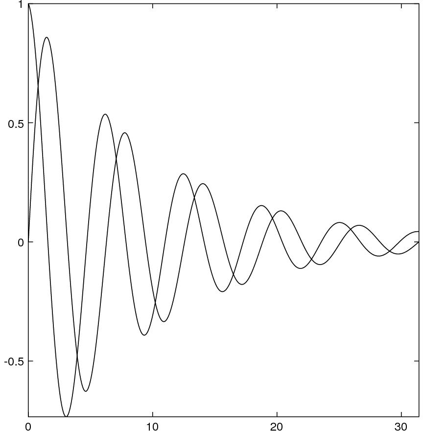
After running the following commands, the graphs of the two functions and will be plotted and saved in the file test.eps.
with("plot.x");
x = linspace(0, 10 * pi, 500);
y1 = cos(x) .* exp(-.1 * x);
y2 = sin(x) .* exp(-.1 * x);
fig = figure.new();
fig.plot(x, y1);
fig.plot(x, y2);
fig.save("test.eps");
a postscript driver with many plotting commands. It is possible to work with these low level routines directly if you're familiar with the postcript language. This class is not documented and you need to look into the source file in order to use it.
2d figure class for creating 2D graphs. There are several attributes corresponding to the the building blocks of figures. All are modifiable. If you want to improve them you can look through the source file.
3d figure class. Draw 2d surfaces and 1d curves in space.
creating bar graphs given a set of data.
creating pie charts given a set of percentages.
Use the following command to create a figure and assign it to a variable named "fig":
fig = figure.new();
plot is an attribute function of figure and can treat two vectors x and y as coordinates of the locations of a sequence of points in the 2d plane. Marks can be drawn at these locations, or lines and curves drawn through them. The command for plotting x and y data on figure fig is
fig.plot(x, y, linetype, linewidth, color, gray);where x and y are two vectors of the same length. The plot can be straight line segements joining the points, marks placed at the locations defined by x and y, or a smooth curve (a piece-wise cubic polynomial) through the dots. The type of the plot is specified by the argument linetype.
| solid | -- | dotty | .... |
| dash | - - - - | dashdot | --.--.--. |
| dot | . . . . | circle | |
| oval | square | ||
| diamond | cross | ||
| flake | asterisk | ||
| triangle | dtriangle | ||
| plus | +++ | curve | (smooth curve) |
linewidth is a number. The line to be drawn will be linewidth times as wide as the default linewidth. For example, to make the line twice as wide as the normal, use value 2.
color is a vector of three numbers between 0 and 1, with each component representing the intensity of red, green, or blue. gray is a number between 0 and 1.
It's not necessary to provide all the arguments to plot. The default values of linetype, linewidth, color, and gray are "solid", 1, [0, 0, 0], and 1. Therefore a simple call
fig.plot(x, y);will draw solid straight line segments through the (x, y) points; the width of the lines is 1 unit, and the color is black. This is because that when calling a function, you may provide only the first few arguments, the others will receive default values. For example,
xx = [0, 1, 2, 3, 4, 5];
yy = [0, 1, 0.5, 0.75, 0.625, 0.6875];
fig.plot(x, y);
To change the line type,
fig.plot(xx, yy, "oval");
To change the line width as well
fig.plot(xx, yy, "oval", 2);
If you just want to specify the line width, you still have to provide at least the first four arguments, but you can use default value for the third argument linetype
fig.plot(xx, yy, *, 2);
Named argument By the previous way of calling fig.plot, the order of arguments have to match the signature of the function. Alternatively, you can use named arguments. For example
fig.plot{x = xx, y = yy, linewidth = 2};
Note that you can not only skip certain arguments, but don't have to follow any
specific order of argument either. For example
fig.plot{y = yy, linewidth = 2, x = xx};
However you still need to provide the correct names of the arguments, namely,
x, y, linewidth, etc.
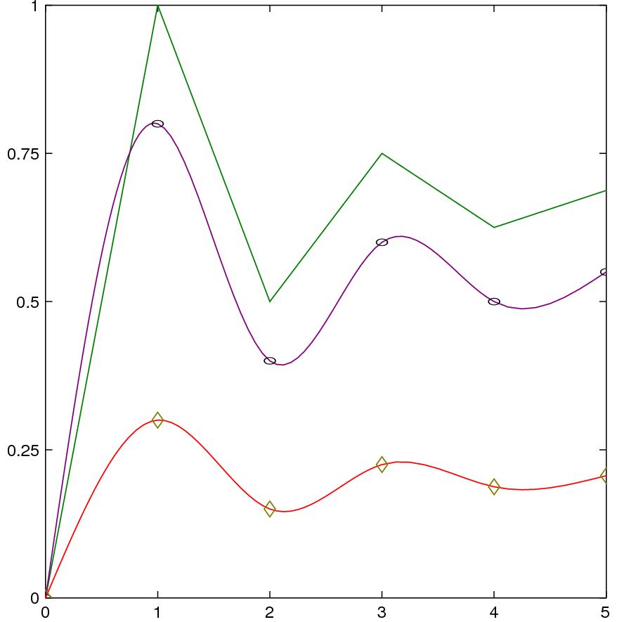
Example
xx = [0, 1, 2, 3, 4, 5];
yy = [0, 1, 0.5, 0.75, 0.625, 0.6875];
fig = figure.new();
fig.plot(xx, yy, *, *, colors.green);
fig.plot(xx, yy*0.8, "curve", *, colors.purple);
fig.plot(xx, yy*0.8, "oval");
fig.plot{x = xx, y = yy*0.3, linetype = "curve", color = colors.red};
fig.plot{x = xx, y = yy*0.3, linetype = "diamond", linewidth = 2, color = colors.olive};
fig.save("symbols.eps");
Some simple shapes can be drawn on the canvas without first defing data.
To draw a line segement you need to specify the starting and the end points.
fig.line(P0, P1, style, linetype, linewidth, color);where P0 and P1 are the starting and end points of the line segement. style is one of "-", "->", "<-", or "<->" which specifies whether one end or both ends of the line has an arrow. linetype is either "solid" or "dotty".
The command
fig.polygon(x, y, type, color);will draw a polygon given the x and y coordinates of the vertices. type can be "contour" or "solid", which specifies whether the polygon is hollow or solid.
The command
fig.rectangle(x, y, width, height, style, cornersize, type, color);will draw a rectangle given the x and y coordinates of the center, the width, and the height. style can be "plain", "rounded", or "beveled", which specifies the shape of the four corners of the rectangle. type can be either "contour" or "solid".
The command
fig.ellipse(ox, oy, a, b, theta, type, color);draws an ellipse. It place the center of the ellipse at the location whose coordinates are ox and oy. a and b are the long and short axes, theta is the angle between the long axis of the ellipse and the horizontal direction of the canavas, type is either "contour" or "solid".
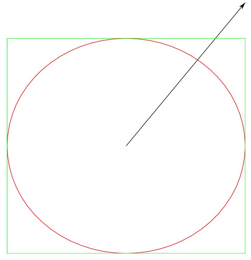
Example
fig = figure.new();
fig.line([0, 0], [2, 2], "->");
fig.ellipse{ox = 0, oy = 0, a = 2, b = 1.5, theta = 0, color = colors.red};
fig.rectangle{x = 0, y = 0, width = 4, height = 3, color = colors.lime};
fig.style = "empty";
fig.save("objects.eps");
A figure has the following attributes that can be modified.
This is the setting surrounding the figure. It can be put in a nice box, can come the horizontal and vertical axes, or coordinate grids. This feature is called the ``style'' of the figure and the value is one of "boxed", "grid", "center", or "empty". To change the style of a figure to "center"
fig.style = "center";
It's the title of the figure, which is displayed on the top. The value should be a string. For example, to set the title of the figure to ``The cosmos''
fig.title = "The cosmos";
The label of the horizontal axis. The value should be a string. To set the xlabel to ``Time"
fig.title = "Time";
The label of the vertical axis. Works the same way as the horizontal axis.
This attribute is a function. It returns the width of the clipping area of the plot. The clipping area is a rectangular box. Anything out of the box is not shown on the actual image. The default values of xrange and yrange would try not to clipp off anything.
To check the xrange of the figure
r = fig.getXrange();
fig.getYrange.() returns the yrange of the clipping box of the plot.
A function attribute. To set the xrange to [-5, 5]
fig.setXrange([-5, 5]);
Similarly to setXrange, fig.setYrange(yr) sets the height of the clipping box to yr, which is vector of 2 numbers.
A character string can be printed anywhere in the graph. The location, size, and other attributes of the text can be specified, but it usually would take some trial and error to get it right or satisfactory. The following is the command for printing text
fig.print(x, y, contents, orientation, alignment, color, font, fontstyle,
fontscale);
where x and y are the coordinates of the location of the text, contents is the text to be printed (a string of characters). The other values are as follows:
| argument | allowed values |
| orientation | "portrait", "landscape" |
| alignment | "left", "right", "center", "top", "bottom", |
| font | "Helvetica", "Times", "Courier", "Symbol" |
| fontstyle | "Regular", "Bold", "Italic", "BoldItalic" |
| fontscale | positive number |
| color | vector of three number between 0 and 1 |
You won't see any picture until you save the figure in a file. To save the figure as an encaspuslated postscript file, do fig.save(filename). For example
fig.save("flowering-times.eps");
Note that most of the processing occurs when the figure is being saved,
therefore if there's something wrong with the plotting commands, error messages usually are not produced until at this stage.
After a figure is saved, it still exists and more contents can be added to it and then it can be saved again.
If you're not satisfied with how a figure looks, you can erase everything in it by using clear. To delete all elements in a figure and leave it empty
fig.clear();Or you could simply redo fig = figure.new() -- the previous value of fig is destroyed.
A color a vector of length three with each element (a number between 0 and 1) representing the intensity of red, green, or blue. Sixteen colors are predefined in the global variable colors.
global.colors = {
     black = [0, 0, 0],
     gray = [0.5, 0.5, 0.5],
     silver = [0.75, 0.75, 0.75],
     white = [1, 1, 1],
     yellow = [1, 1, 0],
     lime = [0, 1, 0],
     aqua = [0, 1, 1],
     fuchsia = [1, 0, 1],
     red = [1, 0, 0],
     green = [0, 0.5, 0],
     blue = [0, 0, 1],
     purple = [0.5,  0, 0.5],
     maroon = [0.5, 0, 0],
     olive = [0.5, 0.5, 0],
     navy = [0, 0, 0.5],
     teal = [0, 0.5, 0.5]
};
To specify a color, one can give the rgb vector like
fig.plot{x = xx, y = yy, color = [0.5, 0.7, 0.2]};
or use one of the predefined colors like
fig.plot{x = xx, y = yy, color = colors.olive};
New color definition can be easily added to the global variable colors. For example:
global.colors.lavender = [0.6, 0.35, 0.73];
fig = figure3d.new();
plot(xf, yf, zf, urange, vrange, meshsize, frontcolor, bgcolor, type);where xf, yf, and zf are the three parameteric equations that define the surface to be drawn. Each of them is a function of two parameters. For example, the unit sphere can be represented by the following three equations
urange is the range of the first parameter. vrange is the range of the second parameter.
meshsize is a vector of two numbers, which specifies how many points are sampled on urange and vrange. If these numbers are big, the surface will be finer and smoother; otherwise it be more like a polyhedron rather than a smooth surface.
frontcolor and bgcolor are the colors of the front side and the back side of the surface respectively. Here we suppose that the surface is orientable, i.e., it has two sides.
type is either solid or contour. If type is solid, the interior of the polygon is painted with the specified color, otherwise only the boundary is painted.
A semisphere can be drawn using this command
fig = figure3d.new();
xf = (u, v) -> cos(u) * cos(v);
yf = (u, v) -> cos(u) * sin(v);
zf = (u, v) -> sin(u);
fig.plot(xf, yf, zf, [-pi/2, 0 ], [0, 2 * pi]);
fig.save("semisphere.eps");
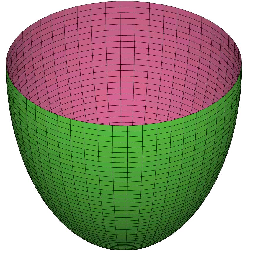
In the above meshsize, frontcolor, bgcolor, and type are not specified -- the default values are used.
Draws a smooth curve through a set of points in the space.
fig.curve(x, y, z, color, lw);x, y, and z are three vectors of the same length which are treated as the coordinates of dots in the space; a smooth curve with width lw through the dots will be drawn. Without some background, it is very hard to tell if a curve is in 3D space. So in the following example, we plot three orthogonal planes to reveal the dimension
fig = figure3d.new();
fig.light_direction = [2/3, 1/3, 3/5];
gx = (y, z) -> 0;
gy = (x, z) -> 0;
gz = (x, y) -> 0;
fig.plot(gx, (y,z)->y, (y,z)->z, [0, 30], [0, 30], [4, 4], rand(3), rand(3));
fig.plot((x,y)->x, (x,y)->y, gz, [0, 30], [0, 30], [4, 4], rand(3), rand(3));
fig.plot((x,z)->x, gy, (x,z)->z, [0, 30], [0, 30], [4, 4], rand(3), rand(3));
t = linspace(0, 10 * pi);
x = 6 * cos(t) + 10;
y = 6 * sin(t) + 10;
fig.curve(x, y, t, colors.red, 3);
fig.save("spiral.eps");
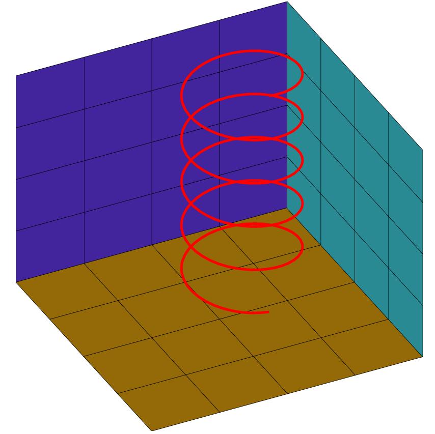
fig.polygon(x, y, z, nv, frontcolor, bgcolor);
Draws a polygon whose vertices are x, y, and z, normal direction is nv (a 3d vector), colors of front and back are frontcolor and bgcolor.
This is like a uniform discretization of a surface over the rectangle . You only need to provide the z coordinates of the points on the surface.
fig.mesh(v, frontcolor, bgcolor);v is a matrix whose elements are treated as the the z coordinates of a set of points. The x and y coordinates are the and .
It's a 3d vector at which the the 3d objects are projected. For example, fig.light_direction = [1, 1, 0.5].
It specifies if the axes are plotted. Choose "boxed" or "empty". For example, fig.type = "empty" will make a graph without axes.
hsr specifies how hidden surface removal is done.
Choose from "auto", "bsp", or "painter". "painter" is more efficient and results in a smaller image size, while "bsp" (binary spatial partitioning) is supposed to render the intersection of the surfaces more accurately. Use fig.hsr = "auto" to let algorithm be automatically selected.
The class is called histogram. To create a memeber of this class
h = histogram.new(xlabels, yvalues, grouplabels);where xlabels is the labels displayed on the horizontal axis used to identify each value. yvalues are the values to be compared. grouplabels is the labels used to identify each group of data. It can be left out if there's only one group.
hist = histogram.new(("a", "b", "c"), ((0.6, 0.25, 0.15), (0.7, 0.32, 0.27), ...
                     (0.9, 0.2, 0.5)), ("Ocean", "Lake", "Pond"));
hist.save("hist.eps");
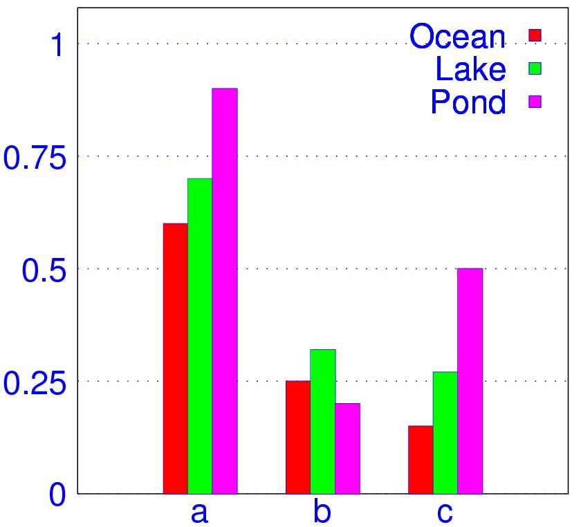
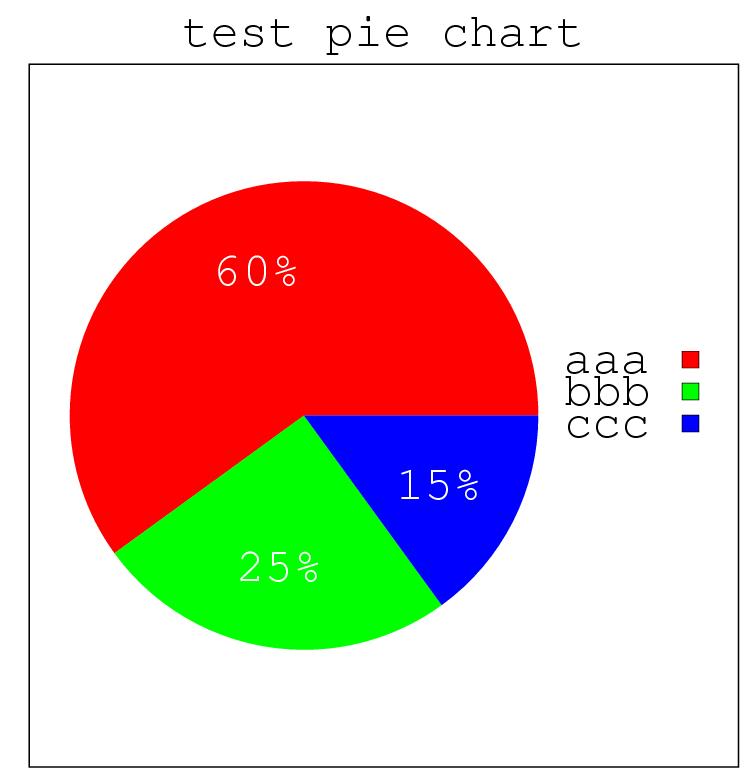
chart = piechart.new(percentages, labels);where percentages is the vector of percentages (must add up to 1), and labels is a list of strings used to identify each percentage.
chart = piechart.new((0.6, 0.25, 0.15), ("aaa", "bbb", "ccc"));
chart.font = "Courier";
chart.save("pie.eps");
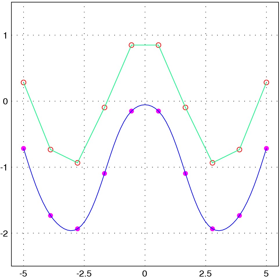
with("plot.x");

     x = linspace(-5, 5, 10);
     fig = figure.new();

     /* draw small circles at (x,y) locations */
     /* color is vector of 3 numbers between 0 and 1, in rgb format */
     fig.plot{x=x, y=cos(x), linetype="circle", color=[1, 0, 0]};

     /* connect the dots with solid lines,
        linetype is the default value "solid" */
     fig.plot{x=x, y=cos(x), color=[0,1,0.5]};

     /* draw circular dots at location underneath the previous curve */
     fig.plot{x=x, y=cos(x) -1, linetype="dot", color=[1, 0, 1]};

     /* connect the dots with smooth curve */
     fig.plot{x=x, y=cos(x) -1, linetype="curve", color = [0, 0, 1]};

     /* set the xrange and yrange of the picutre */
     fig.setXrange([-5.5, 5.5]);
     fig.setYrange([-2.5, 1.5]);

     fig.save("curves.eps");
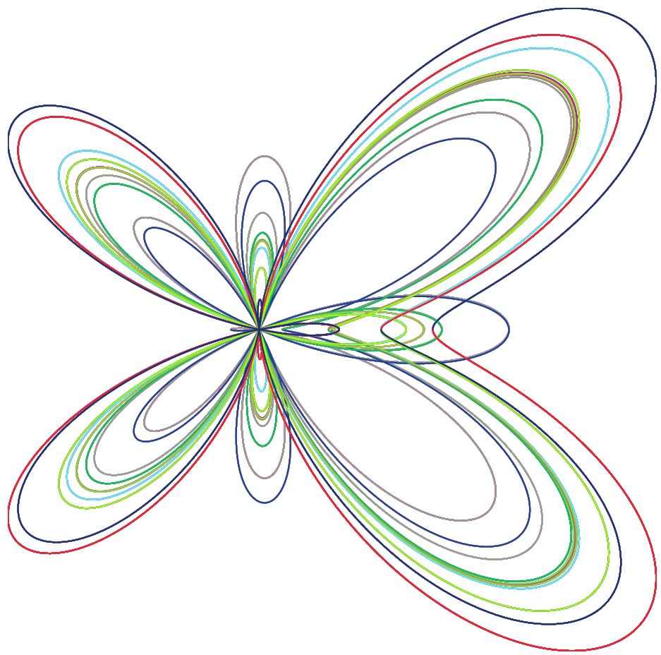
with("plot.x");
fig = figure.new();
for k = 0 : 99
theta = linspace(k * 2 * pi, (k + 1) * 2 * pi, 500);
rho = exp(cos(theta)) - 2 * cos(4*theta)+sin(theta/12).^5;
x = rho .* cos(theta);
y = rho .* sin(theta);
fig.plot{x=x, y=y, linetype="curve", color=rand(3)};
end
fig.style = "empty";
fig.save("butterfly.eps");
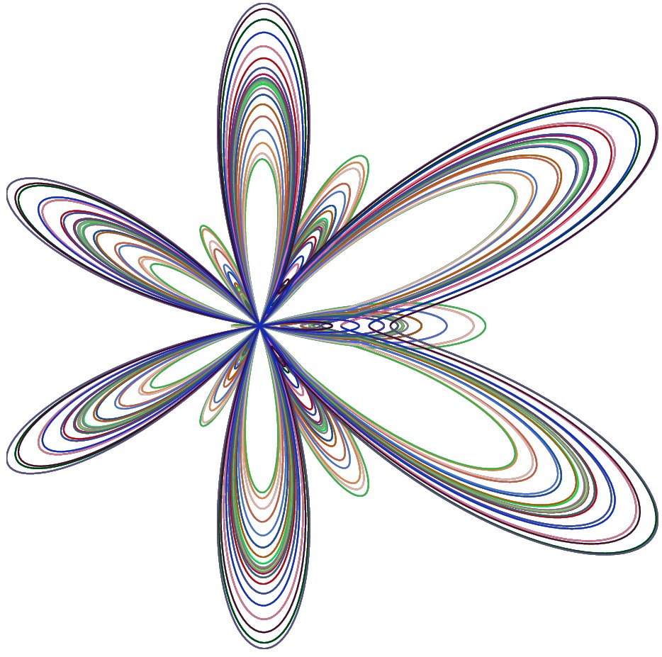
fig = figure.new();
for k = 0 : 99
theta = linspace(k * 2 * pi, (k + 1) * 2 * pi, 500);
rho = exp(cos(theta)) - 2.1 * cos(6*theta)+sin(theta/30).^7;
x = rho .* cos(theta);
y = rho .* sin(theta);
fig.plot{x=x, y=y, linetype="curve", color=rand(3)};
end
fig.style = "empty";
fig.save("butterfly2.eps");
|
|
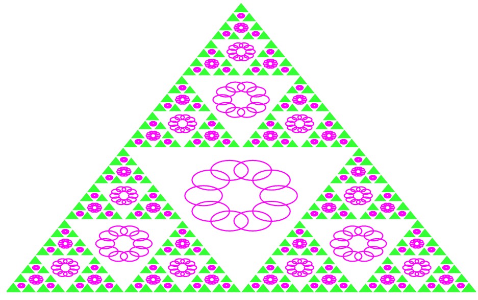
fig = figure.new();

h = 10 * sin(pi/3);
x = [-5, 5, 0];
y = [-h/3, -h/3, h*2/3];

/* the big solid triangle */
fig.polygon(x, y, "solid", [0.2, 1, 0.2]);

/* recursively remove the center of triangle whose vertices are x and y */
/* figp is pointer to fig object. It needs to be a pointer since function
   remove_triangle_center will modify the figure object
 */
remove_triangle_center = function (figp, x, y) -> ()
    L = norm([x[2] - x[1], y[2] - y[1]]);
    xo = x.mean;
    yo = y.mean;

    /* midpoints of the sides */
    xm = [x[1] + x[2], x[2] + x[3], x[3] + x[1]] / 2;
    ym = [y[1] + y[2], y[2] + y[3], y[3] + y[1]] / 2;

    /* [1, 1, 1] is color white -- to remove the center */
	 figp >>. polygon(xm, ym, "solid", [1, 1, 1]);

    theta = pi/5;
    for k = 1 : 10
         cx = xo + L * 0.08*cos(k * theta);
         cy = yo + L * 0.08*sin(k * theta);

         /* draw an ellipse; x and y are center coordinates
                   0.5 and 0.4 are long and short axis
                   0 is angle between long axis and horizontal
                  "contour" is the style -- other option is "solid"
                  [1, 0, 1] is the color -- r=1, g=0, b=1
          */
			figp >>. ellipse(cx, cy, 0.04 * L, 0.03 * L, 0, "contour", [1, 0, 1]);
    end

    if L >= 1
         this(figp, [xm[1], x[2], xm[2]], [ym[1], y[2], ym[2]]);
         this(figp, [xm[2], x[3], xm[3]], [ym[2], y[3], ym[3]]);
         this(figp, [xm[3], x[1], xm[1]], [ym[3], y[1], ym[1]]);
    end
end

remove_triangle_center(>>fig, x, y);

fig.setXrange([-5, 5]);
fig.setYrange([-5, 9]);

fig.title = "Sierpinsky Gasket with flower pattern";
fig.style = "empty";
fig.save("gasket.eps")
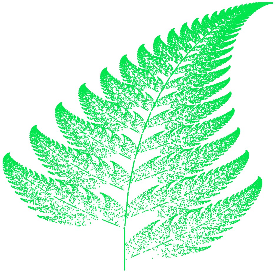
with("plot.x");
N = 50000;

x = zeros(N);
y = zeros(N);
x[1] = 0.5;
y[1] = 0.5;

z = [0.5; 0.5];
p = [0.85, 0.92, 0.99, 1.00];
A1 = [0.85, 0.04; -0.04, 0.85];
b1 = [0; 1.6];
A2 = [0.20, -0.26; 0.23, 0.22];
b2 = [0; 1.6];
A3 = [-0.15, 0.28; 0.26, 0.24];
b3 = [0; 0.44];
A4 = [0, 0; 0, 0.16];

for k = 2 : N
     r = rand(1);
     if r < p[1]
          z = A1 * z + b1;
     elseif r < p[2]
          z = A2 * z + b2;
     elseif r < p[3]
          z = A3 * z + b3;
     else
          z = A4 * z;
     end
     x[k] = z[1];
     y[k] = z[2];
end

fig = figure.new();
fig.plot{x=x, y=y, linetype="dot", linewidth=0.2, color=[0.0, 0.9, 0.3]};
//fig.plot{x=x, y=y};
fig.style="empty";
fig.save("fern.eps");
with("plot.x");
/* generate a tree of n generations */
generate_tree = function (T0, fatom, xatom, n) -> T
T = T0;
for j = 1 : n
t = T;
T = "";
for k = 1 : t.length
if t[k] == "F"
T = T + fatom;
elseif t[k] == "X"
T = T + xatom;
else
T = T + t[k];
end
end
end
end
/*
fatom = "FF-[-F+F+F]+[+F-F-F]";
xatom = "";
T0 = "F";
turning_angle = 22;
*/
/* draw the tree according to commands given in a string
this function is recursive
figp: pointer to the figure object. It needs to be a pointer since
the function will modify the figure object
x, y: the current position
direction: the angle of the current direction
angle: the angle in degree of turning when commands + and - are executed
command: the string of commands
kp: the pointer to the current position in the command string
*/
draw_tree = function (figp, x, y, direction, angle, command, kp, color) -> ()
k = kp>>; /* take the index of the fist command code */
while k <= command.length
c = command[k];
if c == "]"
kp >>= k + 1; /* let kp point to the next command code */
return;
elseif c == "["
kp >>= k + 1;
/* call itself to excute the commands up to the matching ] */
this(figp, x, y, direction, angle, command, kp, color);
k = kp>>;
continue;
elseif c == "+"
direction += angle/180*pi;
elseif c == "-"
direction -= angle/180*pi;
elseif c == "F"
nx = x + cos(direction);
ny = y + sin(direction);
figp >>. line([x, y], [nx, ny], *, *, *, color);
x = nx;
y = ny;
end
++k;
end
end
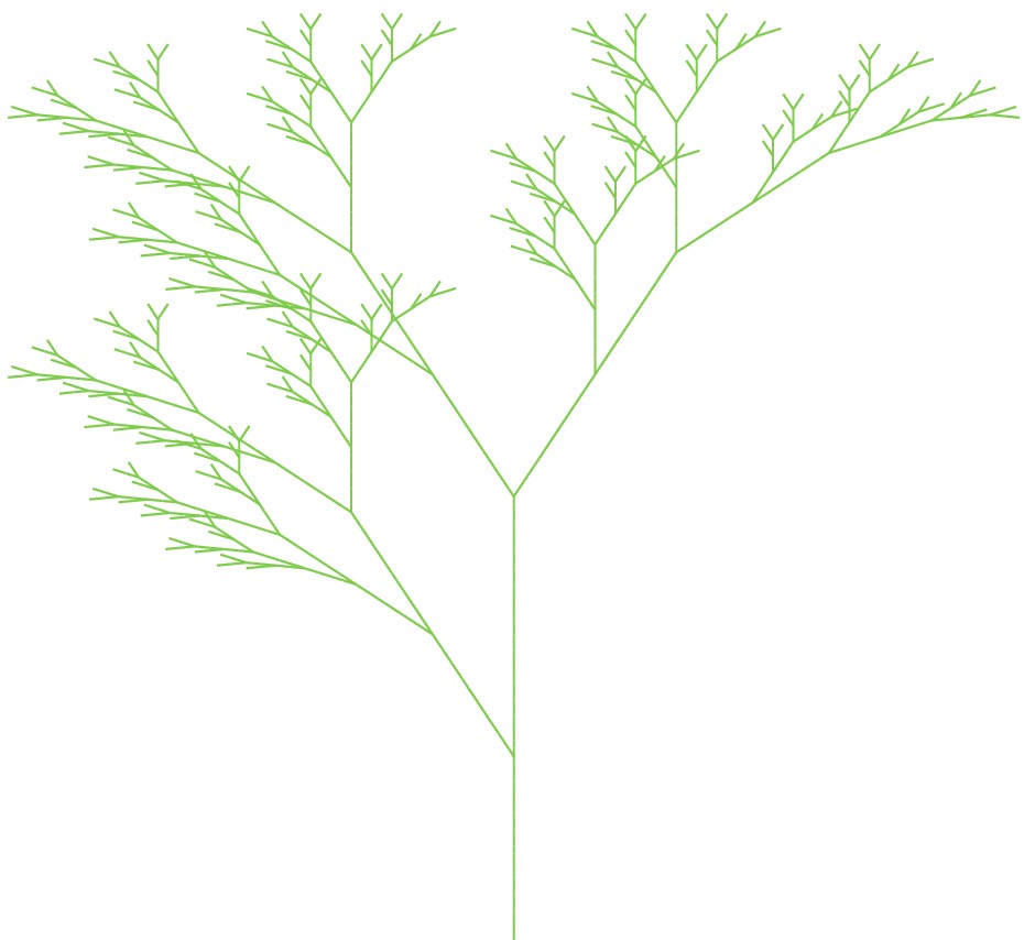
/* ------------- bush 1 ---------------------- */
fatom = "FF-[-F+F+F]+[+F-F-F]";
xatom = "";
T0 = "F";
turning_angle = 22;
bush = generate_tree (T0, fatom, xatom, 4);
/* let command pointer point to the beging of command code sequence */
k = 1;
kp = >>k;
fig = figure.new();
/* pass the pointer to fig to draw_tree */
draw_tree(>>fig, 0, 0, pi/2, turning_angle, bush, kp, colors.lime);
fig.style="empty";
fig.save("bush1.eps");
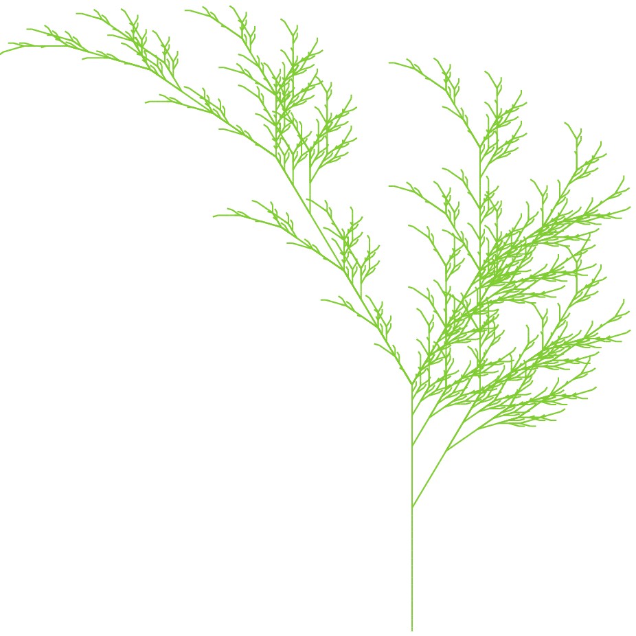
/* ------------- bush 2 ---------------------- */
fatom = "FF";
xatom = "F[+X]F[-X]+X";
turning_angle=20;
T0 = "X";
bush = generate_tree (T0, fatom, xatom, 6);
k = 1;
kp = >>k;
fig = figure.new();
draw_tree(>>fig, 0, 0, pi/2, turning_angle, bush, kp, colors.blue);
fig.style="empty";
fig.save("bush2.eps");
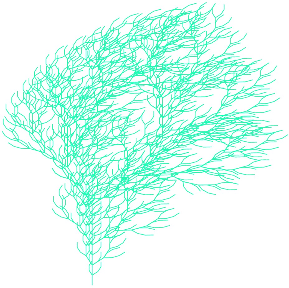
/* ------------- bush 3 ---------------------- */
fatom = "FF";
xatom = "F-[[X]+X]+F[+FX]-X";
turning_angle = 22.5;
T0 = "X";
bush = generate_tree (T0, fatom, xatom, 6);
k = 1;
kp = >>k;
fig = figure.new();
draw_tree(>>fig, 0, 0, pi/2, turning_angle, bush, kp, colors.purple);
fig.style="empty";
fig.save("bush3.eps");
|
|
|
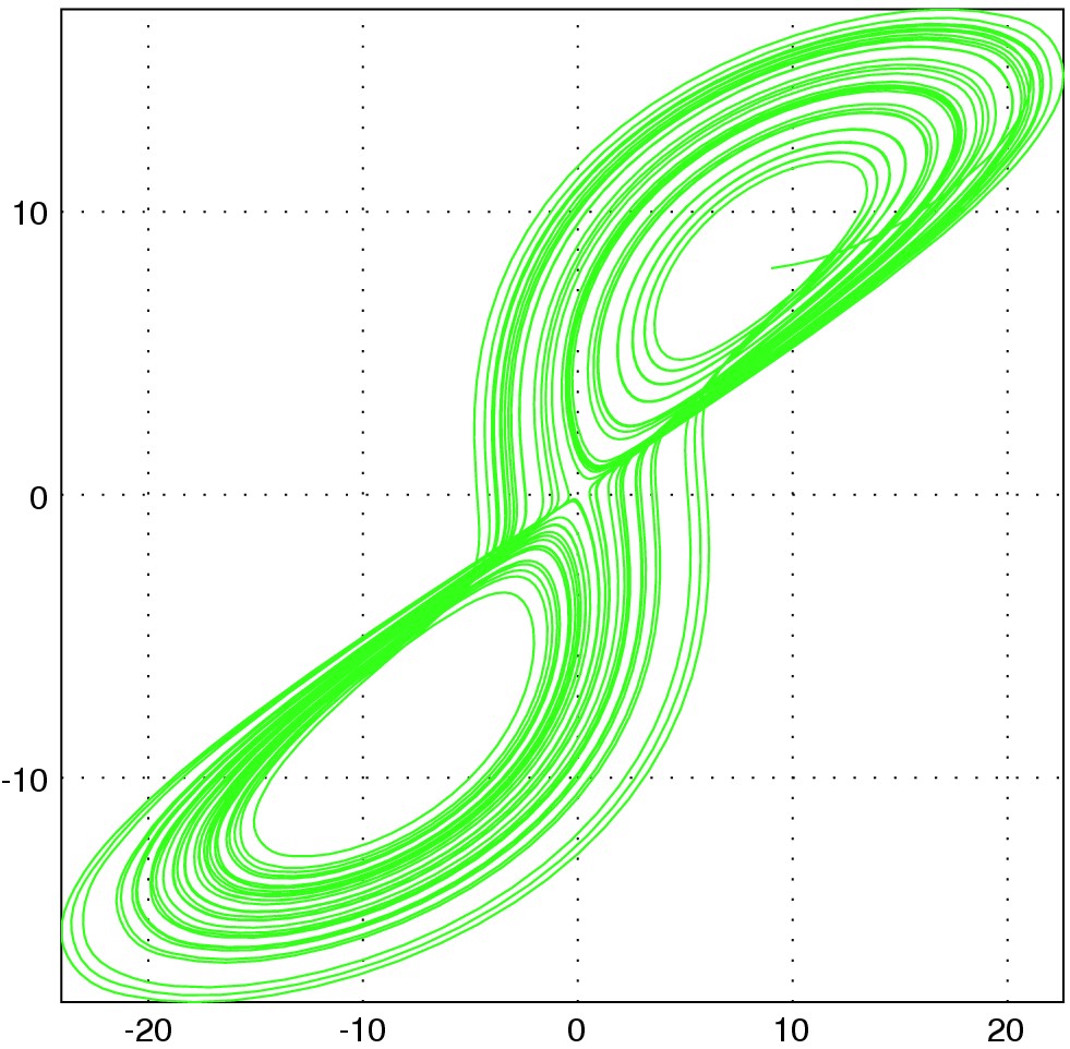
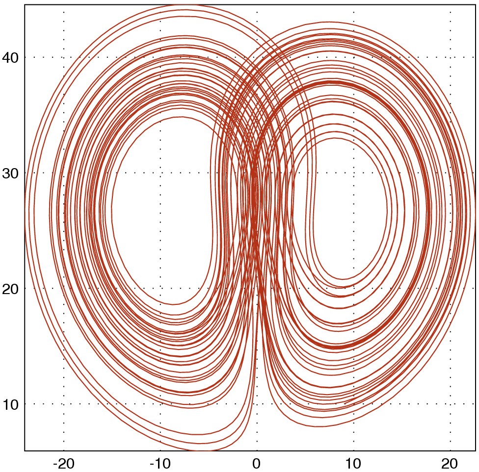
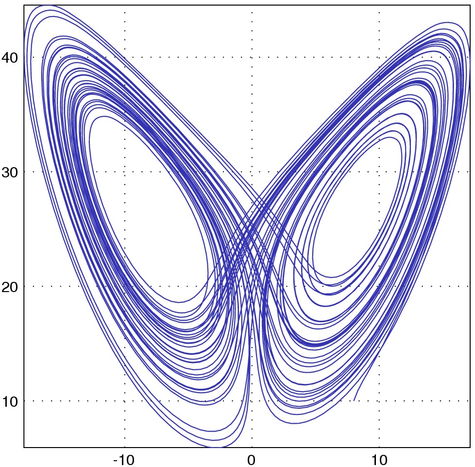
with("plot.x");
/* the lorenz differential equation */
lorenz = function [a = 10, b=28, c=8/3] (t, y) -> dydt
d1 = a * (y[2] - y[1]);
d2 = b*y[1] - y[2] - y[1] * y[3];
d3 = y[1] * y[2] - c * y[3];
dydt = [d1; d2; d3];
end
/* solve the ivp on t=[0,50] */
(x, y) = dsolve(lorenz, [0, 50], [8; 9; 10]);
/* 2d plot */
fig = figure.new();
fig.plot{x = y[:,2], y = y[:,1], linetype = "curve", color = [0.2, 1, 0.1]};
fig.save("lorenz21.eps");
fig = figure.new();
fig.plot{x = y[:,2], y = y[:,3], linetype = "curve", color = [0.7, 0.2, 0.1]};
fig.save("lorenz23.eps");
fig = figure.new();
fig.plot{x = y[:,1], y = y[:,3], linetype = "curve", color = [0.2, 0.2, 0.7]};
fig.save("lorenz13.eps");
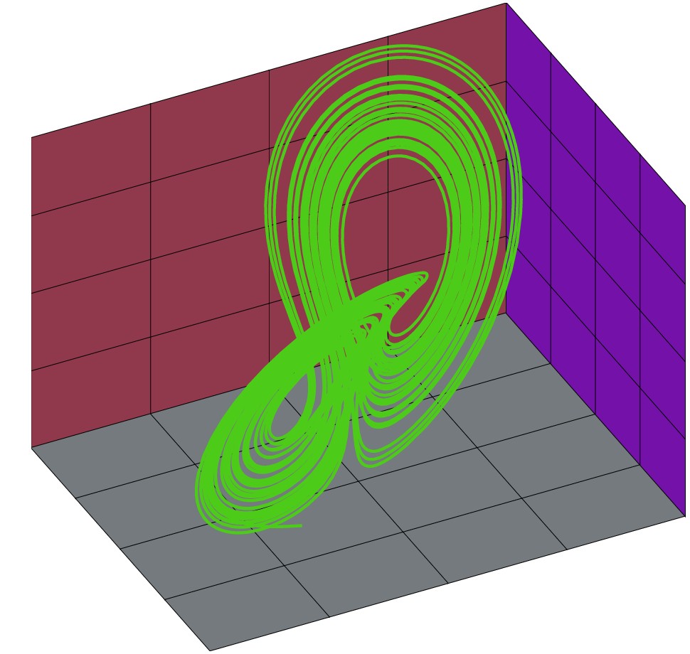
/* for 3d view plot */
cr = y.columnrange;
fig = figure3d.new();
fig.light_direction = [2/3, 1/3, 3/5];
gx = [xv=cr[1,1]] (y, z) -> xv;
gy = [yv=cr[1,2]] (x, z) -> yv;
gz = [zv=cr[1,3]] (x, y) -> zv;
fig.plot(gx, (y,z)->y, (y,z)->z, cr[:, 2], cr[:, 3], [4, 4], rand(3), rand(3));
fig.plot((x,y)->x, (x,y)->y, gz, cr[:, 1], cr[:, 2], [4, 4], rand(3), rand(3));
fig.plot((x,z)->x, gy, (x,z)->z, cr[:, 1], cr[:, 3], [4, 4], rand(3), rand(3));
fig.curve(y[:,1], y[:,2], y[:,3], rand(3));
fig.save("lorenz3d.eps");
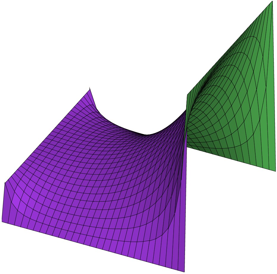
with("plot.x");

// Solve Laplace's equation with Jacob's relaxation method
// Usage: lpc(w,h,bv_up,bv_down,bv_left,bv_right,minchange)
// w: width, h: height, bv_up...bv_down: boundary values, min_change: precision

lpc = function (w, h, bv_up, bv_down, bv_left, bv_right, min_change = 1e-5) -> v

     % a crude guess initial value
     v=(bv_up+bv_down+bv_left+bv_right)*0.25*ones(w,h);

     vave=zeros(w-2,h-2);
     //boundary conditions
     v[1,:]=bv_left*ones(1,h);
     v[w,:]=bv_right*ones(1,h);
     v[:,1]=bv_down*ones(w,1);
     v[:,h]=bv_up*ones(w,1);

     change=10;

     while change>min_change
        vave=(v[2:w-1,1:h-2]+v[1:w-2,2:h-1]+v[2:w-1,3:h]+v[3:w,2:h-1])*0.25;

        change=max(max(abs(vave-v[2:w-1,2:h-1])));

        v[2:w-1,2:h-1]=vave;
     end
end

v = lpc(30,30,5, 5, 9, 25,*);
fig = figure3d.new();
fig.light_direction = [1/3, 2/3, 1/3];
c = rand(3);
d = rand(3);
fig.mesh(v, c, d);
fig.save("laplace.eps");
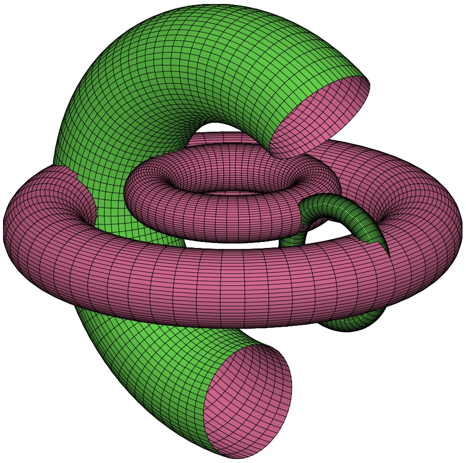
with("plot.x");
fig = figure3d.new();

fx = (theta, phi)->(9 + 2 * cos(phi)) * cos(theta);
fy = (theta, phi) -> (9 + 2 * cos(phi)) * sin(theta);
fz = (theta, phi) -> 2 * sin(phi);

fig.plot(fx, fy, fz, [0,2*pi], [0,2*pi]);

fx = (theta, phi)->(4 + 1.2 * cos(phi)) * cos(theta);
fy = (theta, phi) -> (4 + 1.2* cos(phi)) * sin(theta);
fz = (theta, phi) -> 2+1.2 * sin(phi);

fig.plot(fx, fy, fz, [0,2*pi], [0,2*pi]);

fx = (theta, phi)->1+(9 + 3 * cos(phi)) * cos(theta);
fy = (theta, phi) -> 3 * sin(phi);
fz = (theta, phi) -> (9 + 3 * cos(phi)) * sin(theta);

fig.plot(fx, fy, fz, [0.7,1.2*pi], [0,2*pi]);

fx = (theta, phi)->7+(3 + 0.6 * cos(phi)) * cos(theta);
fy = (theta, phi) -> 0.6 * sin(phi);
fz = (theta, phi) -> (3 + 0.6 * cos(phi)) * sin(theta);

fig.plot(fx, fy, fz, [0,2*pi], [0,2*pi]);


fig.light_direction = [2/3, 2/3, 1/3];
fig.save("torus.eps");
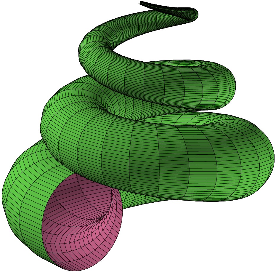
with("plot.x");

/* it's not necessary to use global variable
   in order to use function parameter
	just to show it's possible
 */
global.n = 3;
global.a = 8;
global.b=35;
global.c=5;
fig = figure3d.new();
fig.light_direction = [2/3, -2/3, 1/4];

fx = (s, t)->a * (1-t/(2*pi))*cos(n*t) * (1+cos(s)) + c * cos(n*t);
fy = (s, t)->a * (1-t/(2*pi))*sin(n*t) * (1+cos(s)) + c * sin(n*t);
fz = (s, t)->b * t / (2*pi) + a *(1-t/(2*pi)) * sin(s);

fig.plot(fx, fy, fz, [0,2*pi], [0,6], [50, 50]);

fig.save("seashell.eps");
This document was generated using the LaTeX2HTML translator Version 2002-2-1 (1.71)
Copyright © 1993, 1994, 1995, 1996,
Nikos Drakos,
Computer Based Learning Unit, University of Leeds.
Copyright © 1997, 1998, 1999,
Ross Moore,
Mathematics Department, Macquarie University, Sydney.
The command line arguments were:
latex2html -split 0 plot.tex
The translation was initiated by on 2012-01-14