Xiaorang Li
The goal of design is to make the language very easy to read and learn, and the syntax as intuitive, concise, and clean as possible. Unnecessary keywords, counter-intuitive and complicated syntax rules, and any other kind of inelegant kludges are never introduced into the design.
Shang supports object oriented programming with a number of annovative features. Access to class member attributes can be controlled and member attributes can have domains which protect the integrity of member data and make class interfaces more expressive and readable, and often enough to completely specify the class. Class membership validator and conditional class provide two clean solutions to the well-know "ellipse-circle" difficulty associated with traditional object programming.
Shang is meant to be a gereral-purpose programming language. Yet it is equipped with built-in features for efficiently handling scientific computations, many of which are not found in other popular numerical softwares, such as sets, matrices of infinite size integers and arbitrary precision floating point numbers, internal support for matrices of special patterns such as banded matrices (besides general sparse matrices), handle parameterized functions, etc.
For executing function calls and large loops the Shang interpreter is very fast, compared to other interpreted programming languages (except when the so called Just-In-Time compiler is used; in which case the program is running in compiled mode). This is achieved before any substantial effort is made on optimization. Our next goal is to bring the interpreter close to the speed of compiled languages.
Data types and classes don't form a rigid hierarchical system. A piece of data is usually multi-faceted -- meaning that it is not restricted to the functionality related to a single type and can play different roles. For example, (almost) anything is a function, a function is also a set, a set is also a function, a class is also a set, etc. This often makes it possible to implement functionalities by the most convenient and concise way, yet maintains a uniform interface to the client functions.
Everything including a function and a class is a value and first-class object. Functions and classes can be used anywhere a value is expected. They can be defined inside functions, can be passed to functions as input arguments, and created and returned by functions as outcomes of function calls. New functions can be created not only by writing code, but also by operations on existing functions such as addition/subtraction, multiplication/division, composition, partial calls, and function vector/matrix.
Variables and function input and output arguments may have domains and the language interpreter automatically checks the value of the arguments and generates domain error if the value is not in domain. Shang combines the advantages of both statically and dynamically typed languages. It is as flexible as dynamically typed language, yet it can be more specific than statically typed language, because what it requires is the input argument is inside a domain, not just of a type. A domain is a set that can be defined by different ways, and can be very specific and can often completely ensure the validity of input data, while static typing is often inadequate in this respect.
Functions can have parameters in addition to input/output arguments, which makes functions customizable after they are created, and simplifies the calling sequence in many cases. Functions with parameters act like a class-less objects and spawn new functions like its own constructor.
Shang is objected oriented and has full support for most of the OOP features including access control of member attributes and multi-inheritance. Each attribute of a class can have a domain so that public class attributes can often be used for convenience yet object integrity is still protected. This can help eliminate the need of private attributes and "setter/getters" and make the class interfaces both safe and clean. The attributes a derived class inherited from base classes may violate the validity of the member of derived class. A class may have a validator to guard against illegal actions performed by base class attributes.
Shang has also extended the traditional concept of class to conditional class. A conditional class is a collection of loosely connected objects. Unlike a traditional class, it doesn't ``create'' new members using the constructor, but issues membership to members of other classes that satisfy certain conditions. Such memberships may be cancelled once the conditions are no longer satisfied, or the member can choose to withdraw from the class voluntarily. By using conditional classes, it is possible to avoid unnecessary programming complexity, too many levels of multiple inheritance, and frequent object creations and destructions.
In Shang all the numerical data are consistently represented in matrix format. A scalar is just a one by one matrix. Common matrix operations are supported directly. General data values are also vectorized. Every value is a list; when it is not defined as a list, it is considered a list of one element.
While being a general purpose programming tool, Shang matrices of two and multi dimensions of various storage types including infinite size integers and arbitrary precision floating point numbers for efficient numerical computing. Extensive collection of matrix functions are built-in. Many other constructs such as functions, sets, lists, and tables also make it more convenient and efficient to express computing models and algorithms.
Programing languages that use object references exclusively provide no way to directly handle objects, and cannot do neither passing by value nor passing by reference properly. This promotes implicit behavior of programs and poses particular difficulties when implementing structures like sets which are supposed to maintain a constant value unless changed by their owner. In Shang data values instead of their references are stored in variables therefore a variable's status never changes unless a new value assigned to it, or explicit modifying operation performed on it, and therefore implicit behaviors of programs are reduced. On the other hand, safe and effective pointers are implemented with clear and readable syntax, to provide means to build complicated data structures.
Shang provides automaton - a special data type that is a program with its own variables, whose execution can be halted and resumed, with running status and values of local variables retained. Automatons function as computers and can communicate with each other. They can help implement complicated control flows and event-driven programs.
In the interactive mode the interpreter displays the prompt sign ``»'' to indicate that it is waiting for the user to enter a command.
>>When the user types a command after the prompt and hits Enter, the interpreter will examine the command. If it contains no syntax error and can be carried out, the interpreter will perform some necessary calculations and show the result and display the prompt sign again.
>> cos(pi)
   -1
>>
The interpreter recognizes pi as a system defined global variable that stores the value of the mathematics constant
>> cos(pi)
   -1
>> cos(PI)
   Error: line 2, symbol "PI" not defined
>>
A session can be viewed as a stack whose top level is the interactive mode. If user-defined functions are invoked, the session enters lower levels of the stack. The local variables defined in the interactive mode cannot be accessed on lower levels of the stack. Each level of the stack has its own work space to store local variables and won't interfere with each other. When a function call is finished, the work space is deleted and the active level of the stack is restored to the previous level. For example, during the execution of the following commands, the two variables both named x belong to different levels of stack and won't interfere with each other.
>> x = 10;
>> f = function y -> z
            x = sqrt(1 + y^2);
            z = 1 / x;
       end
>> f(10)
    0.09950371902
>> x
    10
>> (1 + sqrt(5)) / 2
   1.618033989
The value of a^b is ![]() raised to the power of
raised to the power of ![]() .
.
>> 81^(1/2)
    9
Most common elementary functions such as sqrt, exp, log, sin, cos, tan, asin, acos, and atan can be used in the expressions.
Complex numbers are supported directly. A complex number of real and imaginary parts a and b is displayed as a+bi, and can be entered as either a+bi, a+bI, a+bj, or a+bJ. For example
>> sqrt(-5)
    0 + 2.236067977i
>> (3+5i) / (2-3j)
    -0.6923076923 + 1.461538462i
If a constant has the M suffix, it is treated as a multi-precision floating point number. By default, it is stored with 128 binary digits. For example
>> (1 + sqrt(5M)) / 2
   1.61803398874989484820458683436563E0
Expressions that contain a multi-precision floating point number are evaluated with multi-precision. The number of digits of multi-precision computation is controlled by global variable global.mpf_ndights.
>> h = 1.25creates a variable with name h and assign value 1.25 to it. If there is already a variable named h, its old value will be updated to 1.25.
A variable name can be a string of letters and digits, and underscore _, but cannot begin with a digit.
Usually any value can be stored in a variable. But if the domain of the variable is specified, only values inside the domain can be assigned to the variable. For example,
>> h = 1.25 in _D;defines a variable h whose domain is _D, the set of double precision floating point numbers. When the value of h is updated, only values in _D can be used. The domain of a variable can be set only once (when the variable is initialized). The domain can be a finite set, an interval, or any function (which is interpreted as the characteristic function of the set).
>> f = x -> (1 - x) / (1 + x + x^2)A defined function can be called in the usual way
>> f = x -> (1 - x) / (1 + x + x^2)
   user defined function
>> f(-1)
   -2
A function can have several variables
>> f = (r, theta) -> r * (1 + cos(theta));
>> f(2, pi)
   0
More complicated functions have to be defined using the keyword function.
>> h = 1.25;
>>
By suppressing unwanted displays, the command window can be kept cleaner and more efficient.
>> // this is a comment
>> sqrt(-3)   // this is a comment as well
   0 + 1.732050808i
>> sqrt(-3) /* square root of -3 --- this is a comment
               it will be a complex number --- this is still a comment
               the answer is double precision --- yet another comment
               we're now done commenting */

   0 + 1.732050808i
Shang interpreter can recognize five levels of nested multi-line comments.
 f = (h, r, theta) -> r^2 + h * (1 + cos(theta));
 h = 3.5;
 r = 5;
 theta = pi / 2;
 f(h, r, theta)
In the interactive mode, if the following command is issued
>> run("testscript.txt");
   28.5
>>
All the commands in the script file will be executed as if they were just typed in.
 f = (h, r, theta) ->  ...
            r^2 + h * (1 + cos(theta));
>> x = 1011.11    /* decimal format */
   1011.11

>> y = 0B1011.11  /* binary format */
   11.75

>> z = 0X1011.11  /* hex format */
   4113.0664060

>> w = -0Xabcd.ab /* hex format */
   -214375.2578
x = 3.14159265358979323846264338327950MThe default value of mpf_ndigits is 128, therefore an mpf may have 128 significant binary digits (a double has 52 digits). The value of mpf_ndigits. can be set to a multiple (at least 2) of 32.
>> A = [1,4, 9; 2, 3, 5; -2, 5, 10]
   1   4   9
   2   3   5
  -2  5    10
>>
Create Matrices
Alternatively, a matrix of a required size can be created and initialized using built-in functions zeros, ones, or rand. The command
A = zeros(3, 5)will return a matrix of three rows and five columns, with each element being zero. Similar usage of ones and rand will create matrices of 1's and random numbers (between 0 and 1) respectively.
These three functions can also be called with a single parameter, in which case the second parameter is assumed to be 1, and thus a column vector is created.
>> B = rand(5)

    0.289
    0.353
    0.154
    0.566
    0.821
>>
By the dimension of a matrix we refer to the number of rows
and the number of columns. For example, the dimension of the scalar -5 is
   -2    3    9
    10   1    -2
is
Create Even Spaced Vectors Using the Colon Operator
The symbol : can be used to create a row matrix whose elements are evenly spaced. The default step-size of the vector is 1, which is assumed when one colon is used.
>> A = -1 : 5
   -1  0  1  2  3   4   5
To specify a step-size other than 1, two colons are needed.
>> A = 3 : 0.5 : 5
   3  3.5  4  4.5  5
Scalar, vector, and matrix
Every numerical value is treated as a matrix.
It is only for convenience that sometimes we call some special matrices
scalars or vectors.
There is no distinction between
a scalar, a, row or column vector of length 1, or ![]() matrix.
Likewise, a row vector of five elements is the same as a
matrix.
Likewise, a row vector of five elements is the same as a ![]() matrix,
and a column vector of five elements is the same as a
matrix,
and a column vector of five elements is the same as a ![]() matrix.
matrix.
One element or a group of elements of a matrix can be referenced, extracted, or modified by an index expression. An index expression can have a single part, two or more parts separated by commas, or two parts separated by semicolons.
Each part of an indexing expression can be either an integer scalar or a matrix of integers. An index is an integer no less than 1. Zero is not a valid index.
If A is a vector (![]() matrix or
matrix or ![]() matrix), then
A[k] is naturally the kth element of A.
The index doesn't have to be a scalar. If K is a matrix
itself, then A[K] would be a matrix of the same dimensions. For example
matrix), then
A[k] is naturally the kth element of A.
The index doesn't have to be a scalar. If K is a matrix
itself, then A[K] would be a matrix of the same dimensions. For example
>> A = [2, 3, 5, 7, 11, 13, 17, 19, 23];
>> A[3]
      5
>> K = [1, 3, 5, 7];
>> A[K]
      2  5  11  17
>> J = [1, 3; 5, 7]
>> A[J]
    2   5
    11  17
Even if A is not a vector, it is still possible
to use a single index expression to A.
If matrix A has c columns, and
![]() ,
then A[k] refers to the element
of A at
,
then A[k] refers to the element
of A at ![]() -th row and
-th row and ![]() -th column.
In other words, A[k] is the
-th column.
In other words, A[k] is the ![]() -th element of the row vector obtained by
horizontally joining all the rows of A.
-th element of the row vector obtained by
horizontally joining all the rows of A.
>> C = rand(3,5)
    0.802     0.716     0.262     0.752     0.925
    0.65      0.489     0.327     0.859     0.655
    0.396     0.329     0.941     0.854     0.857
>> C[7]
    0.489
>> C[10]
    0.655
The indexing expression can be a matrix itself. In this case a matrix with the same size as that of the indexing matrix is created, whose elements are the elements of the indexed matrix at the positions specified by the elements of the indexing matrix.
A = rand(7)
K = 1 : 2 : 7
A[k]

A = rand(5, 3)
K = [1, 3; 5, 7]
A[k]
If both i and j are scalars, then
A[i, j] refers tot he element of A at ![]() -th row and
-th row and
![]() -th column.
-th column.
When the two indices are not all scalars,
the indexing expression will return a square block of the indexed matrix.
For example,
A[3:5, 7:10] returns a ![]() matrix whose elements are all the elements
of A that lie on rows 3, 4, 5 and columns 7, 8, 9, and 10, namely
matrix whose elements are all the elements
of A that lie on rows 3, 4, 5 and columns 7, 8, 9, and 10, namely
![$\displaystyle \texttt{A[3:5, 7:10]} =
\begin{bmatrix}
\texttt{A[3,7]} & \text...
...[5,7]} & \texttt{A[5,8]} & \texttt{A[5,9]} & \texttt{A[5,10]}
\end{bmatrix}
$](img24.png)
Firstly, if the row and column indices are vectors of the same length, then the two parts form matched pairs - The result of the index expression is a column vector of elements of the indexed matrix whose row and column indices are specified by i and j, namely, the numbers A[i[1], j[1]], A[i[2], j[2]], ...
For example, if both i and j have five elements, then the expression X[i; j] refers to the following matrix
![$\displaystyle \begin{bmatrix}
\texttt{X[i[1], j[1]]}\\
\texttt{X[i[2], j[2]]...
..., j[3]]}\\
\texttt{X[i[4], j[4]]}\\
\texttt{X[i[5], j[5]]}
\end{bmatrix}
$](img25.png)
In particular, if A is a
![]() matrix, then
A[1:6; 1:6] returns the main diagonal of A, and
A[2:6; 1:5] returns the first sub diagonal of A.
matrix, then
A[1:6; 1:6] returns the main diagonal of A, and
A[2:6; 1:5] returns the first sub diagonal of A.
Second, if the length of the row index equals the number of rows of the column index then each entry of row index matches a row of the column index. For example, A[1:3; [1,2,3; 2,3,4; 3,4,5]] would form the following matrix
![$\displaystyle \begin{bmatrix}
\texttt{A[1,1]} & \texttt{A[1,2]} & \texttt{A[1,...
...[2,4]}\\
\texttt{A[3,3]} & \texttt{A[3,4]} & \texttt{A[3,5]}
\end{bmatrix}
$](img27.png)
If the number of columns of the row index equals the length of the column index then each column of row index matches one entry of the column index. For example, A[[[1;2;3],[2;3;4], [3;4;5]]; [1,2,3]] would form the following matrix
![$\displaystyle \begin{bmatrix}
\texttt{A[1,1]} & \texttt{A[2,2]} & \texttt{A[3,...
...[4,3]}\\
\texttt{A[3,1]} & \texttt{A[4,2]} & \texttt{A[5,3]}
\end{bmatrix}
$](img28.png)
In the expression A[\,k], k can be a vector as
well. For example, if A is
![]() , A[\, 1:n-1] would return the elements of the upper triangular
part of A (as a vector).
, A[\, 1:n-1] would return the elements of the upper triangular
part of A (as a vector).
>> A = [1, 2, 3; 4, 5, 6; 7, 8, 9]

   1   2   3
   4   5   6
   7   8   9

>> A[\, 1:2]
   2
   6
   3

>> A[\,1:2] = 0

   1   0   0
   4   5   0
   7   8   9
If A and B are two
If $ appears in the row index of a two-part index expression, its value is m, the number of rows of the matrix; if it appears in the column index, its value is n, the number of columns of the matrix. Therefore, A[$, 2] returns the element at the last row and the second column, and A[1, $] returns the element at the first row and last column.
The dollar sign can participate in arithmetic operations. For example, A[$-2] gives the third last element of A; and A[1 : $, $ - 2] returns the second last column of A. Note that the two $'s have different values in this expression.
>> A = [1, 3, 5, 7, 11, 13, 17, 19];
>> A[9]
   Error 0 "9": index value 9 out of bound 1-8
>> A[9] = 23
   1   3   5   7  11  13  17  19 23
>> A = zeros(5,5);
>> A[2,3]=2.3
>> A[1:3, 1:3] = rand(3,3)
>> A[$]=100
Usually when an index expression is used as an lvalue, the dimension and size of the right hand side of the assignment should match that of the index expression to make the assignment possible. The only exception is when the right hand side is a scalar, then all the indexed elements of the matrix will be set to the same scalar value. For example:
>> A = zeros(3,3)
   0   0   0
   0   0   0
   0   0   0
>> A[1, :] = 3
   3   3   3
   0   1   0
   0   0   1
>> A[\] = 1
   1   3   3
   0   1   0
   0   0   1
When the elements of a matrix are being updated, the indices don't have to be within the upper bounds, which makes it possible to make the size of the matrix grow. As the size of a matrix is extended, the new entries are set to zero, except for those being reset by the assignment statement. For example:
>> X = [1,4,9]
   1   4   9
>> X[4] = 16
   1   4   9   16
>> x[8]=36
   1   4   9    0    0    0   0   36
To create a ![]() int matrix of 0's or 1's, use the command
int matrix of 0's or 1's, use the command
x = zeros(3, 5, _Z);or
x = ones(3, 5, _Z);To create a column vector of 5 bytes of random values between 0 and 255, use the command
x = rand(5, _B);or
x = rand(1, 5, _B);To create a row vector of 5 binaries, use the command binary(5).
sparse and banded matrices use efficient storage scheme and can save on memory, while triangular and symmetric matrices use the same storage scheme as dense matrix and thus woulldn't save on memory but may be more efficient when solving some linear algebraic problems.
Note that these special storage schemes are supported only for double precision floating point numbers.
>> rand(5,3,2);An element or a slice of a multi-dimensional matrix can be referenced or reset using an indexing expression with appropriate number of indices. For example
>> x = rand(5,3,2);
>> x[1, :, :]; // the first slice of x
Note that the only storage type available for multi-dimensional matrices is double precision floating point number. Therefore storage type does not need to be specified.
If two multi-dimensional matrices A and B have the same dimensions, A + B and A - B are defined in the obvious way. The only other operation defined for multi-dimensional matrix is scalar multiplication.
>> s = "During armadillo hunting I picked a diamond ring and dedicated it to my woman warrior."
        During armadillo hunting I picked a diamond ring and dedicated it to my woman warrior.
When using double quotes, the
character \ acts as an escaping signal in order to include special characters
in the string. The defined escaping sequences are the same as provided by the C
programming language. The complete list is given in the table. Note that the
backslash character doesn't have a special meaning in a single quoted string.
| \a | alert (bell) character | \\ | backslash |
| \b | backspace | \? | question mark |
| \f | formfeed | \' | single quote |
| \n | newline | \" | double quote |
| \r | carriage return | \ooo | octal number |
| \t | horizontal tab | \xhh | hexadecimal number |
| \v | vertical tab |
>> x = "Charge, sporky!"
   Charge, sporky!
>> x[7:9]
   , s
>> x[9] = "S"
   Charge, Sporky!
>> x[$]
   !
>> x[9:14] = "Stadum"
   Charge, Stadum!
Note that the $ sign when appearing in an index expression represents the length of the variable being indexed, therefore x[$] refers to the last character of the string.
ASCII values can be assigned to one or several characters of a string. For example,
>> x = "The flying pig"
>> x[12] = 119;
>> x
    The flying wig
>> x[12:14] = [98, 112, 103];
>> x
    The flying bug"
Note that the value assigned to string must be valid ASCII value; in particular,
zero value is not allowed.
When a string s is used as a function, the argument should also be a string t, and the index of occurrence of s as a substring of t is returned.
>> x = "The flying pig";
>> y = "pig";
>> y(x)

   12
>> ["At night", " ", "put", " ", "the cat", "out"]
  At night put the cat out
The same can be achieved by using the addition operator. For example
>> s = "At night" + " " + "put" + " " + "the cat" + "out"
   At night put the cat out
If n is a positive integer and s is a string, n * s or s * n will create a new string which is s repeated n times.
>> s = "RAH RAH AH AH AH ... ";
>> 2 * s
   RAH RAH AH AH AH ... RAH RAH AH AH AH ...
If s and t are two strings of the same length, or one of them has length 1, then s - t returns a row vector of integers, which are the differences between the ASCII codes of s and t. For example
>> s = "bcdefg" - "a"
   1 2 3 4 5 6
>> s = "uvwxyz" - "UVWXYZ"
   32 32 32 32 32 32
If s is a string, and x is a integer scalar, or a vector of integers having the same length as x, then s + x returns a vector of the same length as s whose ASCII values are those of s plus the value(s) of x.
>> s = "BCDEFG" + 32
   bcdefg
Note s - x and x - s are defined in the same manner.
>> s = "bounding" - ("a" - "A")
   BOUNDING
When numbers or vectors are being added to or subtracted from a string, the
resulting must still have characters within the range of ASCII values. Otherwise
the operation is not carried out.
r = ~/zz*/
A few options can follow the closing slash. They are m for multi-line, i for ignoring case, g for finding all matches. When regular expression
r = ~/zz*/giis applied to a string, it will find out all occurences of one or more z or Z's.
A regular expression can be used as either a function, or a set. To match a regular expression r against a string s, just call r as a function:
>> r = ~/zz*/
>> s = "Jazz";
>> r(s)
   3 4
The result is the starting and end indices of the match. If the regular expression also tries to capture substrings, such as /(s)tt*/, then the starting and ending indices of the captured substrings are also returned. If the g option of the regular expression is enabled, the result is a matrix with each row being the information of one match.
Because a function is also a set, so a regular expression can be used anywhere a set is expected, especially for specifying the domain of a function parameter, argument, or a class attribute. For example, the regular expression /zz*/ can be considered as the set of all strings that contain z's.
A regular expression r has the following attributes
The pattern and options attributes can be accessed and reset, and the match attribute is a function that matches the pattern against the argument string, that is, r.match(s) is the same as r(s).
s = ~s/blockhead/simpleton/
Again, a few options can be given after the closing slash. They are m for multi-line, i for ignoring case, and g for finding all matches.
s = ~s/blockhead/simpleton/gi
To apply a regular expression substitution, use it like a function. It doesn't alter the argument string, but returns an updated copy of the string, which can be assigned to the same variable if one wishes.
>> text = "Be prepared for the blockhead persistence";
>> s = ~s/blockhead/simpleton/;
>> text = s(text)
   Be prepared for the simpleton persistence
A regular expression substitution s has the following attributes
The pattern and options attributes can be accessed and modified, and the substitute attribute is a function which does the same thing as s itself.
x = ("fishhook", "gum", "earplug", "lighter");
Any data value can be a list element, including a list. For example
x = (2, [3, 5], x -> sqrt(x^2 + 1), "My goldfish is evil", ("a", "b", "c"));
Here the second element is a matrix, the third element is a function, the fourth
element is a string, and the last element is a list.
To access any element, use the operator # followed by the index. The index value must be an integer starting from 1. For example, the third element is
x#3
Several elements of a list can be indexed at once using a vector index. The result is a still a list. For example
x#[1:3]gives a list of the first three elements of the list, while
x#[1:2:9]returns the list of odd-indexed elements up to the ninth.
To check the length of a list, one can use # followed by the list variable name
>> x = (2, 3, "My goldfish is evil");
>> #x
   3
x.length would achieve the same thing. However, if x is a vector of three elements, x.length would also return 3, while # x returns 1.
The last element of a list can be retrieved using the index $, and the next last using $-1, etc.
Note that Shang is vectorized on the object level. Therefore a list is not a so-called ``container'' in other languages. Any value that is not a list, is actually a list of one item. For example, the number -3 is also a list of one number -3.
x=-3;
y=(-3);
x == y
    1
Likewise, -3, (-3), ((-3)), and (((-3))) are all the same.
And it's impossible to distinguish (a, b) from ((a, b)).
x=("lightsaber", "phaser", "force", ~);
Note that the length of list x is 3, and it is equal to the fixed
length list y=("lightsaber", "phaser", "force"), except that x can be expanded
or shrinked. The tilde at the end of the list is not a special element;
it just signals that the list is capable of changing length. For example
>> x=("lightsaber", "phaser", "force", ~)
   (lightsaber, phaser, force);
>> x#4="schwartz";
   (lightsaber, phaser, force, schwartz);
>> x#6="jam";
   (lightsaber, phaser, force, schwartz, [], jam);
If you plan to create a list x by starting with an empty list and adding new elements one by one, the list should be initialized as
x=(~);Note that both (~) and () are empty list, but new elements can only be added to (~).
List plays a critical role in the operation of functions, as calling a function f with f(a,b,c) is equivalent to the multiplication operation between the function f and the list of arguments (a, b, c).
Variable length lists have the following attribute functions
For both fixed length and variable length lists
anagrams = {"mother in law"       => "woman Hitler",
            "domitory"            => "dirt room",
            "desperation"         => "a rope ends it",
            "election results"    => "lies, let's recount"}
Each element of the table can be extracted and reset
using the operator @.
>> anagrams @ "election results"
   lies, let's recount
Note that a hash table can also act like a function, therefore to reference the entry of a table A with key r, one can use either A@r, or A(r).
If one needs to create a finite function (whose domain is finite set), one doesn't have to write a bunch of code and can use a hash table instead.
>> f = {1 => 0, 2 => 0, 3 => 0, 4 => 1, 5 => 1, 6 => 1};
>> f(1)
      0
>> f(3)
      0
>> f(6)
      1
Values can be reset or added to the table using
A@r = new_value
Note that although both A@r and A(r) refer to the same value of the table, only A@r can be used as an lvalue in an assignment expression.
A hash table can have a default key, which matches anything that is not explicitly used as a key value. For example, if a table is created by
>> u = {1 => 2, 2 => 3, 3 => 4, 4 => 5, default => 0};
Then u(x) = 0 for any x except 1, 2, 3, 4.
colors = {"red", "orange", "yellow", "green", "blue", "purple"}
faces = {1, 2, 3, 4, 5, 6}
To test if a value x is member of a set s, one can use
x (- sor
x in sor
s(x)or
s * xIf x is a member of s, all of the above will return non-zero; otherwise 0.
To add a new member to a set, use
s.add(m)To remove a member from a set, use
s.remove(m)
The k-th element of a set can be extracted using
s[k]However, the order of the members is not a property of the set. Therefore if s[1] is not equal to t[1], it doesn't imply that s does not equal t. Providing the indexing function is for the purpose of looping over the whole set. Note also that set member can not be added or updated using the indexing expression.
>> s = 0 to 1; // interval [0, 1]Note that since any single value is the same as a list whose only entry is that value. Therefore, 0 to 1 is equivalent to (0 to 1), and we can write
>> s = (0 to 1); // interval [0, 1]Open and half open intervals are created using suffix + and -. For example
>> s1 = (0 to 1);   // interval [0, 1]
>> s2 = (0+ to 1-);   // open interval (0, 1)
>> s3 = (0+ to 1);   // half open interval (0, 1]
>> s4 = (0 to 1-);   // half open interval [0, 1)
>> s5 = (0 to inf);   // interval [0, inf)
>> s6 = (-inf to 1);   // interval (-inf, 1]
>> s7 = (-inf to inf);   // interval (-inf, inf) equivalent to _R
>> S = x -> (x >= 0 && x <= 1)
>> 0.5 (- S
     1
>> 1.5 (- S
     0
s (= t
s (< t
s =) t
s >) t
To calculate the union of two sets:
s \/ t
s /\ t
s \ t
All the above three operations can be performed on any objects as well as finite sets. If both operands are finite sets, the outcome is also a finite set. If any operand is not a finite set, the result is usually a function that can be used as a set. For example, if
u = s \/ tthen u is a function such that u(x) = 1 if x is a member of either s or t, and zero otherwise.
The interpreter is capable of determining if s is a subset of t only when s is a finite set. It is done by testing each element of s. If s is defined by a function, such computation is impossible and would not be attempted. The same applies to other set operations that involve infinitely many steps of computations.
s = stack();
To push an item ![]() into the stack,
into the stack,
s.push(x);
To pop the top item out of the stack
x = s.pop();
To check the height of the stack
s.height;
q = queue();
To add an item ![]() into the queue,
into the queue,
q.enqueue(x);
To remove the next available item in the queue
x = q.dequeue();
To check the length of the queue
s.length;
A structure is a group of attribute values with each one associated with an identifier. A structure is created by listing all attributes in a pair of braces. Each attribute is declared and initialized by assigning the value to the attribute name (an identifier), and all attributes are enclosed in a pair of braces. For example
dims = {length = 15, width = 10, height = 9};
Here a structure with three attributes is created. Note that each part of the definition
corresponds to a structure attribute. The identifier on the left side of the assignment sign
declares the name of an attribute, and will not be confused with any local
variable in the
surrounding scope. The expression to the right of the assignment sign is evaluated in
the surrounding scope. For example
     length = 17
     height = 28;
     dims = {length = 15, width = length, height = height};
In definition of the dims structure, when width = length is processed,
width declares a new structure attribute, where length is the value of the
local variable length and has nothing to do with the previously defined attribute
of the same structure, which is also named length.
In height = height, the first height declares a new attribute, while the second will be the
value of the local variable height.
An attribute of a structure can be accessed, added or reset using the dot operator .
>> dims = {length = 15, width = 10, height = 9};
>> dims.height
   9
>> dims.height = 12
>> dims.height
   12
Note that since function is also a data type, attributes of a structure can be functions as well. For example
>> region = {
              shape  = "circular",
              center = [2, -3],
              radius = 15,
              verify = (x, y) -> (x - 2)^2 + (y + 3)^2 <= 225
          };

>> region.verify(3, 2)
   1
One obvious use of structure is to return more than one values in a function. For example
     dstats = function x -> s
                   n = length(x);
                   min = max = sum = x[1];
                   for k = 2 : n
                       sum += x[k];
                       if x[k] < min
                            min = x[k];
                       end
                       if x[k] > max
                            max = x[k];
                       end
                   end
                   mean = sum / n;
                   sd = 0;
                   for k = 1 : n
                        sd += (x[k] - mean)^2;
                   end

                   sd = sqrt(sd / (n - 1));

                   s = {
                          n = n, min = min, max = max,
                          mean = mean, sd = sd
                       };
               end
      x = rand(15);
      dstats(x)
In order to make a copy of a structure, we only need to assign the structure to another variable.
>> dims = {length = 15, width = 10, height = 9};
>> newdims = dims;
>> newdims.width = 30;
>> dims.width
   10
>> newdims.width
   30
A structure encapsulates several pieces of data and behaves like a class member.
One may regard it as an object without a class, or a quicker way to create an
object. Structures lack the more advanced features of classes, but are often
sufficient and more convenient. Another important use of these classless objects
is to provide `candidates' for conditional classes (chapter ![]() ).
They can
``apply'' for memberships of conditional classes and then be able to use the
rich functionalities offered by the classes.
).
They can
``apply'' for memberships of conditional classes and then be able to use the
rich functionalities offered by the classes.
If A and B are matrices of the same dimensions, A + B is a matrix of same dimension whose entries are the sums of the corresponding entries of A and B.
If either A or B is scalar (1 x 1 matrix), then the scalar is added to each entry of the other matrix.
If A is an ![]() matrix and B is
matrix and B is ![]() row vector,
when A+B is calcuated, the
row vector,
when A+B is calcuated, the ![]() th element of B is added to each
element of the
th element of B is added to each
element of the ![]() th row of A.
th row of A.
Similarly,
if A is an ![]() matrix and B is
matrix and B is ![]() column vector,
when A+B is calcuated, the
column vector,
when A+B is calcuated, the ![]() th element of B is added to each
element of the
th element of B is added to each
element of the ![]() th column of A.
th column of A.
If the dimensions of A and B don't match in any of the ways described above, A + B will cause an error. For example
    x = [-2.5, 3; 9, 7]
        -2.5    3
           9    7
    y = [1, -2; 3, -5]
           1    -2
           3    -5
    z = x + y
           -1.5  1
             12  2
If A and B are of the same storage type, then A + B is of the same type. Otherwise the type of the result is same as the one that needs more storage space. For example, if a double matrix and a integer matrix are added, the result is a double matrix.
Subtraction A - B is defined in the similar manner.
>> f = sin + cos;
   f(pi / 4)
        0
>> h = x -> sqrt(x^2 + 1);
>> h1 = f + h;
>> h1(0)
   2

>> g = 2 - sin;
>> g(pi/2)
   2.141592654
Note that the definition of g is
>> M = (3, 5, 9, [2, -3]);
>> N = (1, -7, 0, [-2, 5]);
>> M + N
   (4, -2, 9, [0, 2])
The subtraction of one list from another list is defined similarly. If the lengths of the two lists are different, or if any two corresponding elements can not be added, then the addition of the two lists is undefined and attempt to it will cause an error.
Note that in some languages, adding two lists means concatenating them to make a longer list. In Shang, the operator for concatenating two lists is >-<.
If one of A and B is a scalar and the other is a matrix, the result is a matrix of the same size, whose entries are the products of the value of the scalar and the entries of the matrix. For example
>>   x = 2;
>>   y = -9;
>>   x * y
      -18
>>   A = [3, 5; 2, -8];
>>   3 * A
       9     15
       6    -24
>>   A * 7
       21    35
       14   -56
If A and B are non-scalar matrices, then A * B is the matrix multiplication of A and B. This is defined only when the sizes of A and B match, i.e., the number of columns of A equals the number of rows of B. For example
>>   A = [3, 5; 2, -8; 1, 9];
       3   5
       2  -8
       1   9
>>   B = [2, 1, 7; -2, 0, 8]
       2   1   7
      -2   0   8
>>   A * B
       -4   3   61
       20   2  -50
      -16   1   79
>>   B * A
       15  65
        2  62
Attempt to multiply matrices whose sizes do not match will cause an error.
If A and B are two lists with the same length ![]() , then
A * B is the dot product (A#1) * (B#1) + (A#2) * (B#2) +
... + (A#n) * (B#n).
, then
A * B is the dot product (A#1) * (B#1) + (A#2) * (B#2) +
... + (A#n) * (B#n).
If B is a list of length ![]() , and A is a list whose length
is
, and A is a list whose length
is ![]() and whose each
element is again a list with the same length
and whose each
element is again a list with the same length ![]() , then A * B is the list
of length
, then A * B is the list
of length ![]() : ((A#1)*B, (A#2)*B, ..., (A#n)*B).
: ((A#1)*B, (A#2)*B, ..., (A#n)*B).
If one of A and B is a scalar, while the other is a matrix, then A / B is a matrix of the same size, with each element being A divided by the each entry of B, or each entry of A divided by B, depending which one is a scalar.
If both A and B are matrices, then A / B is the (numerical) solution
of matrix equation X B = A. The matrix B must be an
![]() non-singular square matrix and
A must have n columns. Note that
X B = A is solved numerically, so the solution can only satisfy the equation
approximately.
non-singular square matrix and
A must have n columns. Note that
X B = A is solved numerically, so the solution can only satisfy the equation
approximately.
>>  A = [3, 2, -5];
>>  B = [1, 2, -3; 2, 1, 5; 0, -1, 3];
>>  X = A / B
      11  -4  16
>>  X * B
      3    2  -5
>>  A = [1, 2, -3; 2, 1, 5; 0, -1, 5];
>>  b = [3; 1; -2];
>>  x = A \ b
     0.75
     0.75
    -0.25
>>  A * x
    3
    1
   -2
>> norm(A*x-b)
    2.220446049e-16
Note that
>> A = {3, -5, "abc", 9, 10, -7};
>> B = {9, -3, "abc", -7, -3};
>> A \ B
    {3, -5, 10}
>> A = [1, 2, 3, 4, 5];
>> A .* A
       1   4   9  16  25
>> A = [1, 2; 3, 4];
>> B = [1, 1; 2, 2];
>> A .* B
       1     2
       6     8
>> A ./ B
      1      2
      1.5    2
If the base b is negative and the exponent r
is a fraction, or either b or r is
complex, the result is the principal value of the (multi-valued) power ![]() .
For example
.
For example
  2 ^ (5)
      32
  3 ^ (-2)
      0.1111111111
  9 ^ (1/2)
      3
  (-3) ^ (1/2)
      0 + 3i
If A is a square matrix, and
For example, if we want to square each entry of a vector
>> A = [1, 2, 3, 4, 5];
>> A .^ 2
    [1, 4, 9, 16, 25]
>> B = [-2, -1, 0, 1, 2];
>> A .^ B
    1         0.5       1         4         25
>> 5 % 3
   2
>> 5 % (-3)
   2
.> (-5) % 3
   -2
>> (-5) % (-3)
   -2
>> r = 10 % pi
   0.5752220392
>> (10 - r) / pi
   3
If one of p and q is a matrix and the other is a scalar, or both are matrices of the same storage type, then p % q is defined as a matrix, whose entries are the element-wise modulus of the entries of p and q.
>> x = [1, 5; -5, 1]
>> -x
     -1    -5
      5    -1
(a to b) is closed interval ![]() .
.
(a+ to b-) is open interval ![]() .
.
(a+ to b) is half open interval ![]() .
.
(a to b-) is half open interval ![]() .
.
For example
>> 3+
   3
>> 3-
   3
>> 3 to 5
   [3, 5]
>> 3+ to 5-
   (3, 5)
>> 3 to 5-
   [3, 5)
>> A = [1, 2; -3, 5]
     1      2
     -3     5
>> A'
     1     -3
     2      5
>> v = [1, -5, 3, 2]
     1  -5   3   2
>> v'
      1
     -5
      3
      2
>> U = [2, 3; 2-i, 5-3i]
        2+0i                 3+0i
        2-1i                 5-3i
>> U'
        2-0i                 2+1i
        3-0i                 5+3i
These operations are also defined if either one of x and y is a scalar and the other is a matrix, or both are matrices of the same size. In that case, when the relation of interest is true for any two corresponding elements, the value of the operation is 1. For example
>> 3 > -5
   1
>> -2 >= 0
   0
>> x = [1, 2, 3, 5]
>> x >= 1
   1
>> y = [2, 2, 3, 7]
>> x < y
   0
>> x <= y
   1
There is no special type for logical values. The result of any relational or logical operation is either 1 or 0. To determine if an expression is true, one can use if x. Note that if x==true and if x!=false may not work, because x doesn't have to be equal to 1 in order for it to be true.
>> x = ("abc", "def", "ghi", "jkl");
>> k = 3;
>> if (k >= 1 && k <= #x)
      play(x # k);
   end
>> x = ("abc", "def", "ghi", "jkl");
>> k = 3;
>> if (k < 1 || k > #x)
      "Invalid selection"
   end
>> count = 0;
>> for k = 1 : #x
     if ! (x#k).qualify()
          ++count;
     end
   end
When assignment a = b is carried out, the variable a obtains a copy of b, and the two values are now independent. For example
>> b = (2, 3, 5);
>> a = b;
>> a # 2 = -3;
>> a
   (2, -3, 5)
>> b
   (2, 3, 5)
Two variables can never refer to the same object, or in other words, one object cannot have two different names. This is quite unlike programming languages that store references instead of values in variables.
>> data = (2, 3, "point");
>> (x, y, label) = data;
>> x
     2
>> y
     3
>> label
     point
          A[3] = 5;
          A[1:3] = [-1, 0, 1];
          A[1:3, 1:3] = rand(3,3);
          A[1:3; 1:3] = [3,3,3];
A # 3 = "xx xxx";
A @ "ppp" = 3;
A.name = "flee";
A = A + 3;the variable name A appears twice. The expression reads ``add 3 to A'', and can be written in a condensed form
A += 3;Note that in A += B, A must be a variable or lvalue, while B can be any expression. A += B is a valid statement as long as A + B is defined. For example
>> x = 35;
>> y = 6;
>> x += y + 1;
>> x
    42
>> A = [3, 5, 9];
>> B = [2, 0, -2];
>> A += B .^ 2;
>> A
    7   5   13
There are compound assignment operators for other arithmetic operators, defined
in the same way. They are listed in Table (![]() ).
).
x = x + 1;
y = y - 1;
or
x += 1;
y -= 1;
The expression += 1 has a further shortened form of syntax, which is ++. It can be put in front of or after the variable, i.e., ++A, or A++. The effects of ++A and A++ on the variable A are same, but the values of the two expressions are different, as described below
++A will add 1 to the value of A, and return the updated value of A. -A will subtract 1 from the value of A, and return the updated value of A.
A++ will add 1 to the value of A, and return the original value of A. A- will subtract 1 from the value of A, and return the original value of A.
If ++A and A++ are two stand-alone expressions, their effects on the variable A are same and their own values are discarded, so they are equivalent. But if they are parts of a larger expression, their values will be different. For example:
>> n = 1;
>> p = ++n
   2
>> // now n is 2
>> q = n++;
>> // q is 2
>> // but n is now 3
>> q
    2
>> n
    3
v.aThe attribute name must be an identifier.
Most system defined data types have some built-in attributes. For example, matrices have attributes length, norm, nrows, ncols, etc..
A[index]where A is a matrix of any numerical type. The index can have a single part, or two parts separated by a comma, or two parts separated by a semicolon, or more (3+) parts separated by commas.
Colon Operator for creating evenly spaced vector
If a and b are two real scalar, a <= b, and n is the largest integer such that a+n <= b, then a : b returns a row vector of numbers a, a+1, a+2, up to a+n. If a>b, then a : b returns empty matrix. For example
>> v = 1 : 5
   1  2  3  4  5
>> v = 1.2 : 5.3
   1.2  2.2  3.2  4.2  5.2
>> v = 3 : -1
   []
If a<b are two real numbers, and h>0, then a : h : b returns a row vector of numbers a, a+h, a+2h, up to b, or the largest number a+nh such that a+nh <= b.
If a>b, and h<0, then a : h : b returns a row vector of numbers a, a+h, a+2h, down to b, or the smallest number a+nh such that a+nh> b.
>> v = 1 : 2 : 10
   1  3  5  7  9
>> v = 1.2 : -1 : -5
   1.2   -0.2  -1.2  -2.2  -3.2  -4.2
s # kk must be an integer no less than 1 or a vector whose entries are no less than 1.
The length of a list is obtained by
#s
A.namewhere A is an expression whose value is a function, a structure, a class, or a class member, and name is an identifier.
A@keywhere A is an expression that evaluates to a hash table, and key is an expression whose value is a key of the table.
x in Sor
x (- S
To test if x is an element of a matrix or list S, one can only use
x in STo test if S is subset, true subset, superset, or true superset of a set T, use
S (= T
S (< T
S =) T
S >) T
respectively.
p = >> Aor
p =>> ATo retrieve the value that a pointer p points to, one can use
x = p>>To reset the value pointed to by p, one can use
p>> = new_valueor
p >>= new_value
f * xor
f(x)
When several operators with equal precedence appear in the same statement, they are evaluated according to their associativity. For example, + and - have the same level of precedence and associate from left to right, therefore a-b+c is evaluated as (a-b) + c. The assignment operator = associates from right to left, therefore a=b=c=89 is evaluted as a = (b = (c = 89)).
The following chart shows the order of precedence with the items at the top having highest precedence.
| Operator | Associativity |
| :: | |
| » | |
| . | |
| [], {}, () | |
| #, @ | left to right |
| ' | |
| !, », ++, - | |
| ^, .^ | |
| &*, &/ | |
| *, /, %, .*, ./ | left to right |
| +, - | left to right |
| / | |
| >-<, <->, <-<, >->, => | |
| to, ==, >, <, !=, >=, <= | |
| &&, in, (-, -), (=, =), (<, >) | |
| || | |
| <> | |
| -> | |
| =, +=, -=, *=, .*=, %=, /=, ./=, ^=, .^=, » | right to left |
    if expression
       statement
    end
It is
used to express decisions. When the flow
of program execution comes to an if statement, the expression is
evaluated. If the logical value of the expression is true,
statement will be executed. Otherwise,
statement is skipped and the program moves to the point after end.
For example
 x = rand(2);  // get two random numbers
 // test if the point (x[1], x[2]) is inside the unit circle
 if norm(x) <= 1
    in_circle = 1;
 end
If one wishes to execute certain commands when the expression is true,
and some other commands when its false,
a variant of the if statement that involves three keywords if, else,
and end can be used.
    if expression
       statement group 1
    else
       statement group 2
    end
For example,
 if norm(x) <= 1
    in_circle = 1;
 else
    in_circle = 0;
 end
If the first condition is tested to be false, further condition can be tested
using the elseif keyword
to determine if the second group of commands are to be executed. The following is
the general form of an if statement.
    if expression 1
       statement group 1
    elseif expression 2
       statement group 2
    elseif expression 2
       statement group 2
    ...  // more elseif's
    else
       statement group n
    end
If expression 1 is true, then statement group 1 is executed. If expression 1 is false and expression 2 is true, then statement group 2 is executed. This goes on until the condition after one of the elseif's is true. If none of expression 1 to expression n-1 is true, statement group n is executed.
Note that each statement group can be one or several statements, and can also have nested control structures.
In the general form, the parts that start with elseif and else are optional.
   if ! expression
       command group
   end
Alternatively, one can use the structure unless ... end
        unless expression
            command group
        end
Note that the unless statement only has this one simple form; there can't be any
else or elseif keywords following it.
    for var = k0 : k1
        statement group
    end
where var is a variable name,
k0 and k1 are two expressions that should evaluate to two
integers with k0<=k1.
When the for statement is encountered, the variable var
is set to k0, and if k0 is less than or equal to
k1, the statement group is executed once.
then the variable var is increased by 1. If var is still
within k1, the statement group is executed
again. This is repeated untill var exceeds k1.
The loop counter var is a variable that can be accessed in the group of statements.
It can be either a previously defined variable, or a new name. Inside the loop, the value
of the counter is updated automatically, and therefore shouldn't be altered
explicitly.
Any attempt to modify the value of the loop counter inside the loop results in
an error.
For example, the following code find the sum
![]()
    s = 0;
    n = 1000000;
    for k = 1 : n
        s += k;
    end
A second variant of the for statement
    for var = k0 : step : k1
        statement group
    end
In this case, the loop counter var receives values
of k0, k0 + step, k0 + 2 * step, ..., until it's greater than k1 (if step
is positive), or less than k1 (if step is negative).
Finally, there is a short form of for statement, in which the value of the counter is not needed in the loop, and the code is repeated for a given number of times.
    for n
         statement group
    end
where n should be an expression that evaluates to an integer, which is the number
of times the statement group is going to be carried out.
The statement group of the for loop may contain simple statements or other control structures. For example, the following is a double loop
    A = zeros(10, 10);
    for k = 1 : 10
         for j = 1 : 10
             A[k, j] = k * j;
         end
    end
      while expression
          statement group
      end
What it does is evaluate expression first.
If its logic value is true, the statement group is executed.
Then expression is evaluated again, and if it is still true statement group
is executed again. This is repeated over and over until the value of expression becomes false.
For example:
      s=0;
      k=1;
      while  k <= 100
         s += k++;
      end
The execution of the loop commands should be able to affect the value of the
expression, so that the loop comes to an end at some point. Otherwise,
it will run forever, and the interpreter will have to be closed by the operating
system.
      until expression
          statement group
      end
It is the opposite of while statement. The statement group is executed until
the logical value of expression becomes true.
Note that untill and until are equivalent.
      do
          statement group
      while expression;
It will execute the statement group first and then evaluate the logical
value of expression. If it's false, the loop is over.
If it's true, the statement group will be executed
again, until expression becomes false.
A do-while statement always carries out the statement group at least once.
      do
          statement group
      until expression;
This will execute the statement group first and then evaluate the logical
value of expression. If it's true,
the loop is over. If it's false, the statement group will be executed
again, until expression becomes true.
A do-until statement always carries out the group of statements at least once.
Again, do-untill and do-until are same.
The break statement breaks out of the innermost enclosing for, while, or do loop and continues to execute the statement right after the loop. For example, the following code repeatedly reads a command, and executes the command until the command is "quit", in which case the loop will be terminated.
while 1
   command = readline("Your command: ");
   if command == "quit"
        break;
   end
   execute_command(command);
end
The continue statement skips the rest of the current round of the loop and continues with the next iteration of the loop.
continue statement is very similar to break statement. The difference is it doesn't break out of the loop altogether, but only breaks out of the current round of the loop. Then the interpreter continues to execute the next iteration in the loop.
In the case of a for loop, the loop counter is updated immediately and its value is tested to determine if a new iteration of loop is to be carried out.
For a while or until loop, the execution flow jumps up to the beginning of the loop body. For a do-while or do-until loop, the rest of the commands of the loop body are skipped and execution flow jumps to the loop condition testing.
For example, the following code repeatedly reads and processes a command. If the command is empty, the loop starts over, if the command is "quit" the loop will be terminated. Otherwise the command is executed and new command is read again.
while 1
   command = readline("Your command: ");
   if command == ""
        continue;
   end
   if command == "quit"
        break;
   end
   execute_command(command);
end
Because of the use of continue, no empty string will be
submitted for execution.
	   switch expression
          case value1
               statement group 1
          case value2
               statement group 2
          ...
          default
               statement group
      end
It is equivalent to the following if statement
         if expression == value1
               statement group 1
         elseif expression == value2
               statement group 2
          ...
         else
               statement group
      end
The default clause in the switch statement is optional.
Besides the case keyword, one can also use cases. For example,
      switch word
          case value
               statement group 1
          cases values
               statement group 2
       end
Here, if word is equal to value, statement group 1
will be executed. If
word is not equal to value, but it is a member of the
set values, then
statement group 2
will be executed. It is equivalent to the following if statement
         if expression == value
               statement group 1
         elseif expression in values
               statement group 2
         end
The following code reads lines of text and count the words in them that start
with a, b, c, and d.
   T @ "a" = 0;  // set counters to zero
   T @ "b" = 0;
   T @ "c" = 0;
   T @ "d" = 0;
   T @ "?" = 0;
   while 1
     line = readline("Enter a line: ");  // read a line
     words = split(line, " "); // split the line to a list of words
     for k = 1 : (# words)     // loop over all words
       switch words # k
         cases ~/^ *[aA]/;   // word starts with a or A
             T @ "a" = T @ "a" + 1;
         cases ~/^ *[bB]/;  // word starts with b or B
             T @ "b" = T @ "b" + 1;
         cases ~/^ *[cC]/;
             T @ "c" = T @ "c" + 1;
         cases ~/^ *[dD]/;
             T @ "d" = T @ "d" + 1;
         default
             T @ "?" += 1;
       end
     end
   end
Shang functions are powerful and very easy to use. They also have a number of new features which are not supported in most other programming languages. For example, function can have parameters which make them customizable; their arguments can have domains, so that the interpreter can automatically check if arguments are valid; functions can be added, subtracted, multiplied, and chained to make up new `pseudo' functions; functions can be part of a matrix; a partial list of input arguments can be passed a function to create a new function whose arguments are the ones missing from the list; etc.
A function that can be represented by a single formula can be defined as a
single line map using the symbol ->. For example, function
![]() can be defined by
can be defined by
>>   f = x -> 2*x^2 - 3/x;
>>   f(3)
     17
Here x is the name of the formal argument, and will not be confused
with the variable named x in the surrounding environment (if there is
any) of the
function. The right hand side of -> is an expression involving
constants, the formal argument, and global variables. The local
variables of the surrounding environment are invisible on the right hand side of
->. For example, the code
>> a = 3;
>> f = x -> 2*x^2 - a;
>> Error: symbol "a" not defined
If the function has more than one argument, they can be included in a pair of parentheses. For example
f = (x, y) -> 2*x - y;
If there is no input argument, use a pair of empty parentheses.
>>	f = () -> rand(1)^ 2; //define a function with no input

>> f()    // call it
        0.1156542049
One-linear functions that have no output arguments are useless and
therefore not allowed.
   function input_arguments -> output_arguments
            statement
            statement
            statement
            ...
   end
The first line of a function definition is called the header, which
starts with keyword function, followed by input arguments
and output arguments, which are joined by an arrow ->.
The header must end with a newline, and no other statements can appear in the
line of the header after the output argument.
The last line of the function must be the keyword end.
Between the header and the last line is a sequence of statements.
In the function header, input_arguments and output_arguments are either a single variable name such as x, or a list of variable names, such as (x, y, z), or an empty list. Therefore a function header may look like one of the following
function x -> y  // one input, one output
function (x, y) -> z  // two inputs, one output
function (x, y, z) -> w  // three inputs, one output
function x -> (y, z)     // one input, two outputs
function x -> ()     // one input, no output
function () -> z    // no input, one output
function () -> ()    // no input, no output
Any value is the list containing itself. Therefor x = (x), so function x -> y can be written as function (x) -> (y) as well.
Note that a variable name in the argument list may optionally contain
the default argument value (See ![]() ), and the domain
(See
), and the domain
(See ![]() ) of values of the argument. Therefore, a function header may
look like this
) of values of the argument. Therefore, a function header may
look like this
function (x = 0, y = 1) -> z  // input arguments have default values
function (x = 0 in _R, y = 0 _in _R) -> z  // input arguments have domains
In the examples that follows, only the simplest case are shown- an argument declaration only contains the argument name.
A function definition will evaluate to a value of type function. It doesn't automatically have a name. To be able to call the function, usually we should assign the function definition to a variable, such as
>>  sumto = function n -> s
               s = 0;
               for k = 1 : n
                   s += k;
               end
            end
The above defines a function which takes a single argument n and calculates
the sum of 1, 2, ..., n.
The function is assigned to the variable sumto.
Now we can call the function by using name sumto
>> sumto(100)
     5050
Any variable that is created for the first time (by using assignment statement variable_name = value) in the body of a function definition is a local variable, and can only be accessed by the statements inside the body of the current function definition. Local variables are even not accessible inside the body of a function definition contained in the current function body. For example
f = function x -> y
         var = 35;
         f = function u -> v  // this f is not the previous f
             v = u + var;  // bad, since var is not defined
             ....
         end
    end
The function input and output arguments automatically become
local variables of the function. When the function is called, the input
arguments receive the values passed by the caller, while the output argument
is initialized to null.
The assignment operator = can be used to declare and initialize a local variable, or update the value of an existing variable. The operand on the left side of the = sign is called the lvalue. If the lvalue is an identifier, it must refer to a local variable. If a local variable by that name does not exist yet, a new local variable with this name will be created and initialized. Otherwise the existing variable by that name will be updated. Here we have an example function:
// binary search for target in a list x
binsearch = function (x, target) -> index
                 n = #x;
                 left = 1;
                 right = #x;
                 while left < right
                      // round down using floor
                      center = floor(left + (right - left) / 2);
                      if x # center < target
                           right = center;
                      elseif x # center > target
                           left = center + 1;
                      else
                           index = center;
                           return;
                      end
                 end
            end
It has local variables x, target, index,
n, left, right, center, among which
x and target are input arguments, index is output
argument, and the rest are variables created inside the function body.
When a function definition such as
f = function x -> y
        ...
        ...
    end
is executed, the function definition is processed, and the code is compiled to
instructions in some internal format. But the local variables do not exist until
a call to the function is made. When a function is called, a stack is initialized
that contains all the local variables of this function. Different calls to the
same function will have different variable stacks and therefore different copies
of the local variables.
Upon termination of the function call, all the local variables except for the output argument will cease to exist, the memory they occupy is recycled, and the stack is destroyed. The value of the output argument will be kept and returned to the caller. If the caller chooses to ignore the return value, the interpreter will claim the memory used by the return value - the programmer never needs to worry about `garbage collection'.
taylor_sin = x -> x - x^3 / 6 + x^5 / 120;

test_fun = function x -> d
                 d = abs(sin(x) - taylor_sin(x));
                // bad -- taylor_sin is invisible here
           end
since taylor_sin is a local variable in the scope outside the body of
test_fun and therefore can not be accessed inside.
One solution to this is passing the value of taylor_sin to the
function
test_fun = function (x, f1, f2) -> d
                 d = abs(f1(x) - f2(x));
           end
test_fun(1.25, sin, taylor_sin)
     0.0009258624152
However, this may make the function calls more complicated. Sometimes
there are certain important data values that many functions need to use and
share. It would be convenient to
store such a value in a public area that can be accessed inside any
function.
Such a variable is called a global variable.
The Shang interpreter maintains a global variable that can be accessed anywhere. The name of this global variable is global. It is a structure whose attributes can be used as if they were independent variables. For example, to create and initialize or modify a global variable named volume, one can do
global.volume = 75
To reference a global variable, the keyword and the dot global. can be omitted if the surrounding scope does not have a local variable with the same name. For example
global.taylor_sin = x -> x - x^3 / 6 + x^5 / 120;

test_fun = function x -> d
                 d = abs(sin(x) - taylor_sin(x));
                 /* this will be ok */
           end
test_fun(1.25)
     0.0009258624152
Note that
A global variable can have an optional domain which limits the values that can be assigned to the variable to a set. The domain is declared when the variable is first assigned a value using the keyword in. For example, a global variable defined as follows can only take one of the three values 0, 1, or 2.
global.u = 1 in {0, 1, 2};
After this, an assignment like global.u = 3 will fail and cause an error, since
3 is not in the domain of global.u.
A global variable declaration global.u = 1.5 in 1.5 will
make it a constant.
Note that domain can only be specified once. If domain is not specified when the
variable is created, it has a default domain _ALL, which is the set
of
everything.
If a function does not intend to return any value, then there is no need to specify the output argument variable. The header of the function should look like
f = function x -> ()
       ...
       ...
    end
In this case, the function call f(x) still returns the null
value back to the caller. (the null value is equal to an empty list, or
an empty matrix,
represented the symbol (), or []).
f = function  x -> y
           done = 0;
           ...
           while 1
                ...
                if done
                     y = some_value;
                     return;
                end
                ...
           end
    end
The return statement doesn't take any argument. To let the function call finish and return a certain value, one may assign the value to the output argument prior to the return statement.
To call a function ![]() with argument value
with argument value ![]() , one can write either
, one can write either
f(x)
or
f * x
In other words, you can view the expressions "f of x" and "multiply x by f"
as equivalents.
Conversely, whenever A * B is defined, it can also be written as
A(B).
If f takes more than one input argument, one can either call the function with the correct number of arguments, or call it with a single argument, which is a list whose length is equal to the number of input arguments of the function definition. For example
f = (x, y, alpha) -> (x^alpha + y^alpha)^(1 / alpha);
s = (3, 4, 2);
f(s)   // equivalent to f(3, 4, 2), and f * s as well
On the other hand, if the function definition has only one input argument, it's still possible to call it with more than one actual arguments, in which case, the arguments will be wrapped in a list and the list is passed to the function. This provides a simple way to implement variable argument list.
f = function x -> s
              s = 0;
              for k = 1 : #x
                   s += x # k;
              end
    end

f(2, 3, 5, 7, 11)
    28
In general, no matter how the function f is defined, the signature can be represented as f = function x -> y, where x and/or y can be single variable, list of variable, or empty list.
>> f = g -> abs(g(0));
>> f(sin)
    0
>> f(cos)
    1
The one-linear definition of a function can be used directly
>> f = g -> abs(g(0));
>> f(x -> sqrt(3 + x^2))
    1.732050808
>> select_func = function code -> f
                   if code == 's'
                        f = sin;
                   elseif code == 'c'
                        f = cos;
                   elseif code == 'a'
                        f = sin + cos
                   else
                        f = x -> sqrt(1 + x^2);
                   end
              end
>> f = select_func('a');
>> f(pi/4)
     1.414213562
Also, it is very straightforward to use nested functions -- function definitions inside function definition. For example
create_func = function d -> func
                  ...
                  func = function x -> y
                           y = sqrt(x^2 + 1);
                      end
              end
When create_func is called, it creates a function func
and return it. Note that inside the definition of func, the value of input argument d
is not accessible, so it may seem impossible to create a function based on the
input value of create_func. Actually there are two ways to get around
this - parameterized functions (See
>>  f = function x -> y
               x = x^2 + 1;
               y = sqrt(x);
        end
>>  p = 25;
>>  f(p)
      25.01999201
>>  p
      25
If it is desired to change the value of a local variable using a function,
one can either assign the result of the function call to the variable, or
pass a pointer (See ![]() ) to the function.
) to the function.
>> summary = function x -> (mean, min, Q1, median, Q3, max)
            x = sort(x);
            n = length(x);
            s = x[1];
            min = x[1];
            max = x[1];
            for k = 2 : n
                 if x[k] < min
                      min = x[k];
                 end
                 if x[k] > max
                      max = x[k];
                 end
                 s += x[k];
            end
            mean = s / n;

            global.findmedian = function y -> md
                 N = length(y)
                 if N % 2
                      md = y[(N + 1) / 2];
                 else
                      md = (y[N / 2] + y[N / 2 + 1]) / 2;
                 end
            end

            median = findmedian(x)

            if n % 2
                 Q1 = findmedian(x[1 : (n + 1) / 2]);
                 Q3 = findmedian(x[(n + 1) / 2 : n]);
            else
                 Q1 = findmedian(x[1 : n / 2]);
                 Q3 = findmedian(x[n / 2 + 1 : n]);
            end

       end
>> s = summary([3, 5, 2, 1, 9, 10, 22])
     (7.42857, 1, 2.5, 5, 9.5, 22)
The function returns a single value, which is list of all output
arguments. We can use a multi-assignment statement to pass all the list
assignments to individual local variables of the caller
(mean, min, Q1, median, Q3, max) = summary([3, 5, 2, 1, 9, 10, 22]);
parameter_name = intial_valuewhere parameter_name is a name used to identify the parameter, initial_value is the initial value of the parameter
For example, the following defines a function
![]() , with
two parameter
, with
two parameter ![]() and
and ![]() .
.
   f = function [alpha = 3, beta = 5] x -> y
	         y = alpha * x + beta;
       end
A parameterized function behaves like a class member that has attributes that
can be accessed using the dot operator.
To refer to the value of a parameter alpha of function f outside the function
body (in a scope where f is visible), one can use f.alpha.
For example;
>> f = function [alpha = 3, beta = 5] x -> y
	         y = alpha * x + beta;  // alpha is the value of the parameter
       end
>> f.alpha
   3
>> f.beta
   5
To refer to the value of parameter alpha inside the function
definition body, one can simply use the parameter name, like in the above
example. However, if a local
variable has the same name, the local variable has higher precedence. In this case,
alpha refers to the name of the local variable, while
to access the parameter named alpha, one needs to use
this.alpha.
Of course, this.alpha always refers to a
function parameter, whether there is a local variable alpha or not.
So the above function can also be written as
   f = function [alpha = 3, beta = 5] x -> y
	         y = this.alpha * x + this.beta;
       end
Inside a function body, the keyword this refers to the function itself.
The following example illustrates the difference between a local variable and
a parameter.
>>   f = function [alpha = 3, beta = 9] () -> y
            alpha = -5;   /* now alpha is a local variable */
            y = [alpha, this.alpha, beta, this.beta];
     end
>>   f()
       -5    3    9    9
>> f = function [public alpha = 3, public beta = 5] x -> y
         y = alpha * x + beta * y;
   end
>> f.alpha
   3
>> f.alpha = -5;
>> f.alpha
   -5
>> f.beta = 10;
>> f.beta
   10
It's impossible to change the value of a public parameter inside the function
body. For example, if we do
>> f = function [public alpha = 3, public beta = 5] x -> y
            alpha = 10;
            ...
       end
>> f.alpha
        3
we merely creates a local variable whose name is alpha and value is 10. And
>> f = function [public alpha = 3, public beta = 5] x -> y
            this.alpha = 10;
            ...
       end
will result in an error, since this.alpha is not modifiable inside the
function. The purpose of this restriction is to reduce the
implicit behavior of a function. The owner (the surrounding scope) of a function can always predict the
behavior of a function as long as it only has public parameters because the
function itself cannot change the values of its public parameter.
>> f = function [private count = 0] x -> y
            this.count = this.count + 1;
            ...
   end
>> f.count
   0
>> f(1);
>> f.count
   1
>> f(2);
>> f.count
   3
>> f.count = 0; // !!! error ...
Inside the function body, to modify a private parameter, this
keyword must be used.
Private parameters cause the function to behave implicitly, and make
the results of the function call hard to predict, therefore
they should be used only when necessary.
A readonly parameter is an attribute of the function that is accessible but not modifiable inside and outside the function. However, its value can be modified by other common or auto parameters.
common and auto parameters are both functions
A common parameter is an attribute of the function that is itself a function. Its value is fixed (to the initial value, which is a function). It is like a utility function which can be used to reset the values of readonly parameters.
An auto parameter is an attribute of the function that is itself a function which takes no input arguments. When the auto parameter is accessed, the function will be called automatically.
The following example will illustrate the uses of various parameters.
polynomial = function [private coeff,
       common  setcoeff = function c -> ()
                             parent.coeff = c;
                          end,
       auto roots = () -> polyroots(parent.coeff)] x -> y

       y = polyeval(coeff, x);
end
Here polynomial is an implementation of polynomial function. Suppose
the system has a builtin-in function polyeval such that given a vector
of coefficients c and a number x,
polyeval(c, x) returns
![]() . Then
polynomial function can be used like this
. Then
polynomial function can be used like this
f = polynomial;
f.setcoeff([1,2,3]);
f(10)   // ans is 321
f.roots
roots is an auto parameter, therefore f.roots is equivalent to f.auto().
>> plot = function [coordinate = "cartesian" in {"cartesian", "polar"},
                 color_scheme = "bw" in {"bw", "rgb"}] (x, y) -> ()
                ...
                ...
       end
>> plot.color_scheme = "rgb"; // ok
>> plot.color_scheme = "bs";  // !!! error
The general syntax for specifying the domain of a parameter is
[access_control_type] parameter_name [= initial_value [in domain]]where initial_value is the initial value of the parameter, domain is the domain of the parameter. initial_value and domain are evaluated in the scope surrounding the function definition. If the domain is specified, then the value assigned to the parameter must belong to the domain. Otherwise an error will occur.
The value of domain may be a finite set, which is defined using a pair braces, like in the above sample function plot. Domains can also be functions that act like sets. For example, we may use the following function to define a set of positive numbers
positive = x -> (x > 0);Then we may use this function as the domain of a parameter
lf = function [alpha = 1 in positive, beta = 0 in positive] x -> y
          y = alpha * x + beta;
     end
Note that the set positive can be represented using interval
positive = 0+ to inf, or using the built-in function _R.
By using domains we ensure that parameters can only be set to valid values, and then the function is never in an illegal state. Note that although you don't have to provide a domain in the function definition, every parameter always has a domain - the default domain for any parameter is the set that contains everything - _ALL. Since anything belongs to this set, having it as domain won't apply any restrictions to the values assigned to the parameter.
g = f;will create a copy of f and assign it to g. Any modification to g will not affect f. Only functions that have parameters are modifiable. The following code makes a copy of f and then modifies the copy.
f = function [alpha = 1] x -> y
         y = sqrt(x^2 + alpha^2);
    end
g = f;
g.alpha = 5;
Now we have two functions
Any function can act as a prototype and new functions can be ``spawned'' directly from it. The syntax of spawning a new function is
f[parameter_value_1[, parameter_value_2, ...]]where parameter_value_1 is the value of the first public parameter, parameter_value_2 the value of the second public parameter, etc. The parameter names must appear in the same order as in the original function definition, with non-public parameters skipped. For example
f = function [alpha = 1] x -> y
         y = sqrt(x^2 + alpha^2);
    end
g = f[5];
g will be a function that is the same as f, except that
its parameter alpha has value 5.
It's possible to combine function spawning and calling and pass the values of arguments and parameters at the same time. For example
>> f = function [alpha = 1] x -> y
         y = sqrt(x^2 + alpha^2);
   end
>> f[5](3)
   5.830951895
   fac = function n -> f
               if n <= 1
                    f = 1;
               else
                    f = n * this(n - 1);
               end
         end
Inside the function body, this refers the function fac,
therefore this(n - 1) is a call to the function itself.
The result of calling fac(n) will be the factorial of n, i.e.,
the product of 1, 2, ..., up to n.
This appears to be a neat solution for doing recursion, but it cannot be used
to implement indirect self-calling.
In this case the best strategy is to define the
functions as global variables.
The following is an example of indirect recursion.
   global.f = function x -> y
                 ...
                 global.g(3);
                 ...
              end
   global.g = function x -> y
                 ...
                 global.f(3);
                 ...
              end
Here the two functions f and g call each other. We call this
indirect recursive function call. Note that direct recursion can be done like
this as well.
   global.fac = function n -> f
               if n <= 1
                    f = 1;
               else
                    f = n * fac(n - 1);
               end
         end
Note that the statement f = n * fac(n - 1) can be written as
f = n * global.fac(n - 1) as well.
Finally, it's also possible to implement recursion by passing the function to itself as an input argument value (or set it to one of its parameter values). For example:
>> fib = function (n, f) -> s
                if n <= 1
                     s = 1;
                else
                     s = f(n - 1, f) + f(n - 2, f);
                end
   end
which can be called as follows
>> fib(10, fib)
   89
f = (x, y) -> exp(-(x^2 + y^2)) * sqrt(x^2 + y^2);we don't have to pass the values of both arguments to f all at the same time. Instead, we may pass the value of y to f, and leave x unspecified. The result is a new function of x. An unspecified argument value is represented by a dot.
f1 = f(., 3)Here the definition of function f1 is
In general, when a function is called, some input arguments can receive dots, while the rest receive actual values. The result of such a function call is a new function whose input arguments are those of the original function that receive dots, while the arguments of the original function which do get values passed to are no longer arguments of the new function. Here a dot means a missing or delayed value, and corresponds to an argument of the new function. Calling the new function is equivalent to calling the original function by two separate steps of argument passing. For example:
>> f = function (x, y, alpha) -> s
           s = (x^alpha + y^alpha) ^ (1 / alpha);
    end

>> f2 = f(., ., 2);
>> f2(3, 4)    // equivalent to f(3, 4, 2)
   5
A function call in which all argument values are dots will have no effect - it
just evaluates to the original function. For example, sin(.) is the same
as sin.
With the support of partial substitution, we can write a general function, which takes all the relevant arguments. For a particular application, all calls to the master function may use a set of fixed values for some arguments. Then we may create a customized version of the function by partially substituting these often used argument values into the function. The calling sequence of the customized function is more compact. For example, a plotting function may be designed to take all the following arguments
plot = function (x, y, coord, line_style, color,
                            axis, xlabel, ylabel) -> graph
                 .....
                 .....
       end
If every time we use the same choice of coord, line style,
color,
axis, xlabel, and ylabel, then we can do
myplot = plot(., ., "cartesian", "solid", "bw", "boxed", "population", "revenue");to make a plotting function that takes only x and y as arguments.
Partial substitution provides an alternative way to function parameters for customizing the behavior of a function after it is created. Unlike parameterized functions in which some variable are predefined to be parameters, in partial substitutions any of the input variables can be chosen as parameters. However, in terms of performance it may be at disadvantage compared to the function parameter approach since one more abstract level is added and two argument passing steps have to be processed in order to perform a call to a partial substitution.
>> f = function (x = 3, y = 5, z = 7) -> w
       // define function w = f(x,y,z), with
       // default argument values 3, 5, 7
         ...
   end
>> f(*, 10, *)   // equivalent to f(3, 10, 7)
Here the default values of the 1st and 3rd arguments are passed to the function.
Function calls don't have to match the signature of the function definition exactly. To be specific, there are the following situations.
Another fact is that every function argument has a default default value. The default default value of an input argument is null (which is the same as the empty matrix []). For example, if the definition of function f starts with f = function(x, y, z) -> w, then function call f() is equivalent to f(null, null, null). Of course, unless the function definition code does something to handle default default value, using it directly will usually cause an error.
The domain of an argument is specified in the function header using the following syntax
variable_name = default_value in domain
For example, the function header may look like
global._RP = (0+ to inf);
func = function (x = 1 in _RP,
           options = "real" in {"real", "complex") -> y in _RP
    ...
end
The above defines a function that takes two arguments x and
options. _RP is the set of all positive numbers. So the
argument x must be a positive number, while options must be
either "real" or "complex". The output argument value
y must be a positive number as well. Whenever func is called
with invalid input argument values, the interpreter will complain.
>> func(-5, 6) // !! domain error ...
When function definition is processed, the default value and the domain of an argument are evaluated in the scope surrounding the function definition. Therefore they can be expressions containing the local variables of the surrounding scope, but they cannot make an reference to the other argument names of the function definition. For example
x = 3;
p = function (x = x) -> (y = x)
        ...
    end
Here in (x = x) -> (y = x), the first x is the name of the formal
argument, while the second and third x refer to the value of the local
variable x (whose value is 3) of the surrounding scope.
We may define a set, and then use it as the domain in a function definition immediately
Dmx = x -> (x <= -1 || x >= 2);
Dmy = x -> (x >= -1 && x <= 2);

f = function (x = 3 in Dmx, y = 0 in Dmy) -> z in _RP
           ...
    end
In practice sometimes the domains of two arguments are not independent of each other. For example
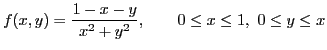
Dxy = v -> (v in _R2 && v[0] >= 0 && v[0] <= 1 && v[1] >= 0 && v[1] <= v[0]);

f = function v = [1, 1] in Dxy -> w
           w = (1 - v[0] - v[1]) / (v[0]^2 + v[1]^2);
    end
Note that if the domain of an input argument is given, a default value must be provided. Otherwise the interpreter may find the default default value (= null) does not belong to the domain, and have difficulty processing a call to the function that provides default argument value. On the other hand, one may specify the default value but omit the domain. Whenever the domain is not specified, a default domain, which is _ALL, the set of everything, will be set as the domain of the argument.
Programming languages can roughly be divided into two categories: statically typed, in which argument value must be of a certain type, and dynamically typed, in which formal arguments can be any type. Shang has both the flexibility of dynamically typed language and the rigorousness of statically typed language. It is in fact superior to statically typed language with respect to type-checking since the domain is a set, which can be much more expressive and specific than a type. Many times, being a value of certain type doesn't guarantee that the argument is a valid one. For example, if an argument a represent age. Statical type checking only guarantees that a is an integer, while in Shang, the domain of a can be a customized set that contain all valid ages, such as integers between 0 and 150.
f{x=3, y=9}
Here x and y must be the same formal argument names declared in
the definition of the function.
Calling functions this way has two advantages. Firstly, the order of the arguments doesn't matter. For example f{x=3, y=9} and f{y=9, x=3} would be the same. Secondly, you don't have to pass a value for every argument. Any arguments not named in the braces will take default values (specified in the function definition).
Note that an expression {x=3, y=9} is exactly the same as the syntax for defining a structure with fields x=3, y=9. So passing arguments as named parameters is similar to passing a structure to the function.
>> x = rand(5, 1);
>> length(x)
     5
>> cos(pi/4)
     0.7071067812
The complete list of the built-in functions is given in the appendix.
Like user-defined functions, built-in functions can have parameters as well. For example, the built-in function normal which generates (pseudo) random numbers of normal distribution has five parameters mu, sigma, pdf, prob, and quantile. mu and sigma are the mean and standard deviation of the distribution.
>> normal(1)
    0.5723149278
>> normal(2)
    1.64
    -0.559
>> normal.mu
    0
>> normal.sigma
    1
>> normal.prob(-inf, 0)
    0.5
The two parameters mu and sigma are modifiable.
Their initial value are mu = 0 and
sigma = 1 respectively. If we want a non-standard normal distribution
random number generator, we may make a copy of normal and reset the
values of mu and sigma
>> my_normal = normal;
>> my_normal.mu = 10;
>> my_normal.sigma = 2;
>> my_normal(1)
      8.029350953
>> my_normal(2)
      12
      10.9
>> my_normal.prob(-inf, 10)
      0.5
Note that normal is a global variable and can only be modified using
the global keyword, therefore normal.mu = 10 doesn't work
while global.normal.mu = 10 does.
In my_normal = normal, normal does refer to the global
variable normal, since it is not an assignment statement.
The assignment my_normal = normal assigns a copy of
global.normal to my_normal, which can then be modified.
It's very easy to override the definition of a built-in function. Locally defined variables have higher precedence. Once they are defined, they will replace the built-in definitions.
>> sin = x -> x - x^3 / 6;
>> sin(6)
     -30
However, an overridden built-in function is not lost. Actually all built-in functions
are attributes of the global variable builtin. So they can always be
accessed using builtin.name. For example
>> sin = x -> x - x^3 / 6;
>> sin(2.5*pi)
    -72.891530550
>> builtin.sin(2.5*pi)
    1
The operators for function addition and subtraction are + and
-, while the
operators for function multiplication and division are &* and &/
respectively. The operator for function composition is <>.
| Operator | Definition |
| h = f + g | f(x) = f(x) + g(x) |
| h = f - g | f(x) = f(x) - g(x) |
| h = f &* g | f(x) = f(x) * g(x) |
| h = f &/ g | f(x) = f(x) / g(x) |
| h = f <> g | f(x) = f(g(x)) |
| h = -f | f(x) = -f(x) |
For f <> g, the number of output arguments of g should be the same as the number of input arguments of f.
For example
>> f = sin + cos;
>> f(pi/4)
    1.414213562

>> p = sin &* cos;
>> p(pi/4)
    0.5

>> g = sin - cos;
>> g(pi/4)
    -1.110223025e-16

>> h = log <> sin;
>> h(pi/2)
    0
Note that in the above, f and g don't have to be both
`real' functions - they can be pseudo functions, or anything that can be used
as functions, such as numbers or matrices. If either operand is a function, the operation will create
a new pseudo function. For example
f = sin + 2will create a function f(x) = sin(x) + 2x. Note that 2 as a function means x -> 2x instead of x -> 2.
f = [cos, -sin; sin, cos];defines a function
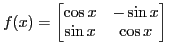
>> f = [cos, -sin; sin, cos];
>> f(pi/4)
    0.707    -0.707
    0.707     0.707
Note that the elements of the matrix can be data of other type that can be used
as functions, and are not restricted to
functions (user or built-in). As long as one element is a function, the whole
matrix is evaluated to a function matrix. The following example creates a
function matrix
f = [exp <> cos, 2; x -> sqrt(1 + x^2), exp <> (-sin)]which represents the following function
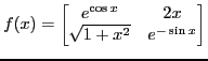
In general, all the elements of a matrix function should have the same number of input arguments, and the return values should be compatible for building a matrix.
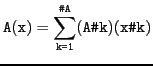
f = {0 => 1, 1 => 2, 2 => 3, 3 => 4, 4 => 5, 5 => 0};
>> s = floor(rand(5) * 10)
    5
    3
    0
    7
    2
>> fs = s[.];
>> fs(1)
    5
>> fs(3)
    0
Another example
>> s = floor(rand(5, 5) * 10)
    7         0         5         8         3
    9         0         3         7         8
    1         6         6         7         9
    2         5         5         3         2
    1         2         5         5         0

>> fr = s[., :];
>> fr(1)
   7         0         5         8         3
>> fr(3)
   1         6         6         7         9
>> fc = s[:, .];
>> fc(1)
     7
     9
     1
     2
     1
>> fc(3)
     5
     3
     6
     5
     5
Sometimes a structured set of data is stored most efficiently in a vector or
matrix. However a client function that needs to use the data may expect a function
that returns one data item given an index.
In such a situation we can store the data in a matrix A, and pass A[.]
whenever the client function is being called.
A class is a set whose members are data values `created' by the set itself. Each member of a class is a structural value whose attributes are prescribed in the class definition. A class definition includes a constructor, which is a function used to create new class members, and specifications of other member attributes. When a new class member is created by calling the constructor, the member will possess the member attributes. Member attributes can be any data type including functions. An attribute function may access or modify the other attributes of the member.
     class
          attribute_1;
          attribute_2;
          attribute_3;
          ....
          attribute_N;
     end
There are two types of attributes, those for the members of the class and those for the class itself. They are called member attributes and collective attributes respectively.
To define a member attribute, one needs to specify the type of access control
access_control_type identifier [= default_value [in domain]]
where the specification of default_value and domain is
optional.
A collective attribute definition starts directly with the name of the attribute
(Only three such attributes are allowed now: new, base, and title).
   circle = class
              public radius = 1;
              auto   perimeter = () -> 2 * pi * parent.radius;
              auto   area = () -> pi * (parent.radius)^2;
            end
in which radius is a public attribute, and perimeter
and area are two auto attributes. If x is a
circle, then one can use x.radius to find its radius, and use
x.radius = new_value to reset its radius to a new value.
The new value assigned to a public attribute must belong to the
domain of the attribute, which, by default, is _ALL.
Inside an attribute function, to access another attribute of the same member of the class, the keyword parent must be used. In the above example, if x is a member of circle class, then in the surrounding scope of x, the radius of x is x.radius, while inside an attribute function (such as perimeter and area) of x the radius of x is referred to as parent.radius.
>>   circle = class
              private radius = 1;
              common  getRadius = () -> parent.radius;
              common  setRadius = function x  ->  ()
                          if x > 0
                             // accessing radius attribute is ok here
                             parent.radius = x;
                          end
                      end
              auto    perimeter = () -> 2 * pi * parent.radius;
              auto    area = () -> pi * (parent.radius)^2;
            end
>>   p = circle.new();
>>   p.radius;  // Error: accessing private attribute
>>   p.getRadius()
       1
>>   p.setRadius(12);
>>   p.getRadius();
       12
Here radius is private attribute and cannot be accessed outside the
class. But other attribute functions (getRadius and
setRadius) can access it using the parent keyword.
In the previous example, the two functions getRadius and setRadius are common attributes. Common attributes as functions can be called outside or inside the class, but they cannot be modified. For example
>>  circle = class
      ...
      common  setRadius = function x  ->  ()
        if x > 0
            parent.radius = x;
         end
      end
      ...
    end
>>  p = circle.new();
>>  p.setRadius = function x -> ()
         ...
    end

    Error: modifying common attribute
If setRadius is declared as public, then we can still use it
almost the same way, but we'll be free to assign new values to the setRadius attribute
of any individual member of circle.
	auto f = function () -> y
                   ...
                   ...
            end
Suppose that u is a member of a class that has an f attribute.
The value of an auto attribute cannot be modified, therefore
u.f = new_value is not allowed.
To call an auto function, one can use
either u.f() or simply u.f.
If f were a common attribute, the would have to be called by
u.f().
For example
   circle = class
              public radius = 1;
              auto   perimeter = () -> 2 * pi * parent.radius;
              auto   area = () -> pi * (parent.radius)^2;
            end
If x belongs to the circle class, to find its area, one only
needs to write x.area. But manually setting x.area to
new value using x.area = new_value is not allowed, since
x.area can only be automatically calculated using the attribute function.
The syntax for specifying the domain of an attribute is the keyword in followed by a set.
   global._RP = (0+ to inf);
   circle = class
              public radius = 1 in _RP;
              auto   perimeter = () -> 2 * pi * parent.radius;
              auto   area = () -> pi * (parent.radius)^2;
            end
Here _RP is a global variable predefined to be the interval of all positive scalars. With this domain
specified, now only positive numbers can be assigned to the radius
field.
When an attribute is declared without specifying a domain, its domain will be the default value _ALL, which is the set of everything. Note that whenever a domain is specified, the default value of the attribute must also be specified, since the default constructor of the class will create a member of the class that has only default attribute values. Then if the attribute has a domain but no default value, and the domain doesn't include the null value, the constructor may return an invalid object.
Domain is most useful for public attributes. In the following example,
each attribute of a person is public, and therefore can be
accessed and modified directly. Yet, only valid values can be assigned to the
attributes. In many languages, to protect the integrity of data, such
attributes must be made private, and direct access to them disallowed.
Instead, function attributes called ``getters'' and ``setters'' are used to
access and modify their values (see the example in ![]() ).
).
person = class
              public gender = "M" in {"F", "M"};
              public age = 1 in 1 : 150;
              public first = "Jerry" in ~/[A-Za-z][A-Za-z]*/;
              public last = "Gallo" in ~/[A-Za-z][A-Za-z]*/;
         end
Although domain makes most sense in the case of public field, a private
field can have a domain as well.
    global.circle = class
          base = global.ellipse;
          title = "circle";
          new = radius -> ();

          public radius = 1 in _RP;
          auto longaxis = () -> parent.radius;
          auto shortaxis = () -> parent.radius;
          auto area = () -> pi * (parent.radius)^2;
          auto perimeter = () -> 2 * pi * parent.radius;
    end
A very simple and effective way to write a constructor is to write a one-liner function. For example
   student = class
             public name = "xxx xxx";
             public id = "000000";
             public age = 18;
             ...
             new = (name, id, age) -> ();
             end
At first sight, the constructor may appear to be doing nothing at all. Actually, when the constructor is called with three input arguments, a function stack is created which has three local variables named name, id, and age. The values of the three local variables are the arguments passed to the constructor when it's called. Because all these three names are also names of member attributes of the class, a class member is created whose name, id, and age attributes obtain the corresponding values of the input arguments of the constructor.
In this example the constructor simply uses the input arguments as values of member attributes without any checking. If one would like to manually check the validity of the input arguments, one can write some code in the constructor to do so. If the checking fails, error can be generated and new class member is not created. Note that if the definition of each member attribute has a domain, then even if the constructor does no explicit value checking, the domain-checking is still performed. Therefore a simple constructor like the above one may still be sufficient.
In the absence of a constructor, when the class definition is processed the interpreter will generate a default constructor. When the default constructor is called, it will create a member of the class all of whose attributes have default values. Note that the default constructor is equivalent to
         class
             ...
             new = () -> ();
             ...
         end
   student = class
             public name = "xxx xxx";
             public id = "000000";
             public age = 18;
             ...
             new = function args -> ()
                        if #args == 3
                             name = args # 1;
                             id = args # 2;
                             age = args # 3;
                        elseif #args == 2
                             name = args # 1;
                             id = args # 2;
                        else if #args == 1
                             name = args;
                        end
                   end
             end
The base of a class is specified in the definition by specifying the base collective attribute. For example:
   global.person =   class
                       public name = "???";
                       public dob = "???";
                       public gender = "F";
                       ...
                     end

   global.student =  class
                       ...
                       base = person
                     end
Here person should be a value visible in the surrounding scope of the definition of student class. Usually it should be a globally defined class name. To avoid potential name clashes, one can use
base = global.person
Now student is a derived class of person, all attributes defined for person will be created for any member of student as well. For example
   >> s = student.new();
   >> s.name  // check s's name, which is inherited from 'person'
   >> s.dob   // check s's dob, which is inherited from 'person'
There is no language facility provided for calling the constructor of the base class automatically. The derived class needs a constructor to handle the initialization of the inherited attributes.
The private member attributes of base class are not accessible to the attribute functions of the derived classes.
base = {s1, s2, s3}
If there is a name conflict, the keyword as can be used to clarify which class is referred to. For example, if m belongs to both aggressor class and philanthropist class, and both classes have member attribute strength, then one can use (m as philanthropist).strength or (m as aggressor).strength to eliminate the ambigulty.
A class may have a common attribute validate which verifies that the state of the class member is valid. Whenever an attempt to modify a class member is made, the modification will be temporarily made and then validate is implicitly invoked. If it returns non-zero value, the validation is passed and the modification will take effect. Otherwise, the modification will be reversed.
Note that validate is called whenever an update of class member state is made. If x.a must equal to x.b in order for x to be valid, a simultaneous assignment (x.a, x.b) = (v, v) must be done in order to pass validation.
global.ellipse = class
        title = "ellipse";
        public a = 1 in (0 to inf);
        public b = 5 in (0 to inf);
        auto longaxis = () -> max(parent.a, parent.b);
        auto shortaxis = () -> min(parent.a, parent.b);
        auto area = () -> pi * parent.a * parent.b;
        new = (a, b) -> ();
end

circle = class
        base = global.ellipse;
        title = "circle";
        auto radius = () -> parent.a;
        auto longaxis = () -> parent.radius;
        auto shortaxis = () -> parent.radius;
        auto perimeter = () -> 2 * pi * parent.radius;
        common set_radius = r -> ((parent.a, parent.b) = (r, r));
        common validate = () -> (parent.a == parent.b);
        new = (a, b) -> ();
end

u = circle.new(3, 3)
u.a = 5; // won't work
(u.a, u.b) = (5, 5)  // this will be OK
Note that without the validate function, u.a = 5 will change
u to an ellipse with a = 5, b = 3.
    >>  Dog = class
                 .....
                 .....
            end

    >>  Spot = Dog.new();

    >>  Spot in Dog   // check if Spot is a member of the dog class
              1
    >>  Person = class
                 ...
                 public dog in Dog;
                 ...
        end
Here a member of the Person class has an
attribute dog, which has to be a member of the
Dog class.
The member of a class is naturally the member of all the base classes of this class.
The operators that can be overloaded are +, -, *, /, .*, ./, ^ , [], ., including the dot operator.
To overload an operator, a member attribute with a specific name needs to be
defined. The operator and the attribute names are given in table
(![]() ).
).
If class s is defined as follows
s = class
         common _sum = y -> z
			          ...
                end

         common _sqbracket = i -> z
			          ...
                end

         common _dotmul = y -> z
			          ...
                end

         common _field = str -> z
			          ...
                end
    end
and x is a member of class s, then
x+y is the outcome of x._sum(y),
x[i] is the outcome of x._sqbracket(i),
x[i, j] is the outcome of x._sqbracket2(i, j),
x .* y is the outcome of x._dotmul(y),
and
x.str is the outcome of x._field(str).
The following example illustrates the usage of operator overloading. It is a simple implementation of sparse matrix class. Note that Shang does have built-in support for sparse matrix, which is much more efficient and feature-rich.
sparsemat = class
     private index = [1, 1];
     private y = 0;

     readonly nrows = 10;
     readonly ncolumns = 10;
     readonly size = 100;
     readonly nzn = 0;

     new = function (nrows, ncolumns) -> ()
                 size = nrows * ncolumns;
           end

     common _subasgn = function (n, y) -> ()
               if n >= 1 && n <= parent.size
                    indx = [fix((n - 1) / parent.ncolumns) + 1, (n - 1) % parent.ncolumns + 1];
                    for k = 1 : parent.nzn
                          if parent.index[k,:] == indx
                                if y == 0
                                    parent.index[k,:] = parent.index[parent.nzn, :];
                                    parent.y[k] = parent.y[parent.nzn];
                                    --parent.nzn;
                                else
                                    parent.y[k] = y;
                                end
                                return;
                          end
                    end

                    ++parent.nzn;
                    parent.index[parent.nzn, :] = indx;
                    parent.y[parent.nzn] = y;
               else
                    panic("index out of bound");
               end

            end

     common _subasgn2 = function (idx1, idx2, y) -> ()
               if idx1 >= 1 && idx1 <= parent.nrows && idx2 >= 1 && idx2 <= parent.ncolumns
                    indx = [idx1, idx2];
                    for k = 1 : parent.nzn
                           if parent.index[k,:] == indx
                                if y == 0
                                    parent.index[k,:] = parent.index[parent.nzn, :];
                                    parent.y[k] = parent.y[parent.nzn];
                                    --parent.nzn;
                                else
                                    parent.y[k] = y;
                                    return;
                                end
                           end
                    end

                    ++parent.nzn;
                    parent.index[parent.nzn, :] = indx;
                    parent.y[parent.nzn] = y;
               end
            end

     common _sqbracket = function n -> y
               if n >= 1 && n <= parent.size
                    y = 0;
                    indx = [fix((n - 1) / parent.ncolumns) + 1, (n - 1) % parent.ncolumns + 1];
                    for k = 1 : parent.index.nrows
                          if parent.index[k,:] == indx
                                y = parent.y[k];
                                return;
                          end
                    end
                    y = 0;
               else
                    panic("index out of bound");
               end

     end


     common _sqbracket2 = function (i, j) -> y
               if i >= 1 && i <= parent.nrows && j >= 1 && j <= parent.ncolumns
                    y = 0;
                    for k = 1 : parent.index.nrows
                          if parent.index[k,:] == [i,j]
                                y = parent.y[k];
                                return;
                          end
                    end
                    y = 0;
               else
                    panic("index out of bound");
               end

     end

     common _mul = function x -> b
          if parent.ncolumns == x.nrows && x.ncolumns == 1
               b = zeros(parent.nrows, 1);

               for k = 1 : b.nrows
                    v = 0;
                    for j = 1 : parent.ncolumns
                         v += parent[k, j] * x[j];
                    end
                    b[k] = v;
               end
          end
     end

     common _sum = function x -> b
          if x in type(parent) && parent.nrows == x.nrows && parent.ncolumns == x.ncolumns
               T = type(parent);
               b = T.new(parent.nrows, parent.ncolumns);
               for k = 1 : x.nrows
                   for j = 1 : x.ncolumns
                        b[k, j] = parent[k, j] + x[k, j];
                   end
               end
          end
     end
end
A.attrib_name = value;For example
x.color = "red";
Acquired attribute definition may also carry a domain.
x.color = "red" in {"red", "gree", "blue"};
Specification of domain can occur only at the first time the attribute is
defined (the first time a value is assigned to the attribute). If domain is not
given, the attribute will have the default domain, which is the set
_ALL.
Subsequent assignment to the attribute can no longer specify a new domain, and
the assigned value must belong to the domain of the attribute.
A structure is an object which doesn't belong to any class. It therefore has no class attribute and only has acquired attributes. To define such an object, just enclose all attributes in a pair of braces.
solution = {x = 3.8, y = -5.2};
New acquired attributes can be added to the object and updated at any time, and domain can be specified when it's added for the first time.
It is worth mentioning here that the keyword global is actually a structure that can be accessed in any scope. The attributes of global function as global variables.
A conditional class is a collection of loosely connected objects. Unlike a normal class, it doesn't ``create'' new members using the constructor, but issues membership to members of other classes that satisfy certain conditions. Such memberships may be cancelled once the conditions are no longer satisfied. An object can easily obtain the memberships of many different conditional classes.
By using conditional classes, it is possible to avoid unnecessary programming complexity, too many levels of multiple inheritance, and frequent object creations and destructions.
Besides the utility attributes, a conditional class may have a number of common or auto member attributes. These are the member services provided by the class. Note that the first argument of any of the attribute function is always the class itself, so that there is never a need to resolve name conflict between different conditional classes. When an object tries to use any of the member services, validate will be called. Only upon success of validate, the service can be provided.
The following code defines an ellipse, a regular class and circle, a conditional class.
The validate function of circle tests if a value x is an ellipse and if x.a is equal to x.b.
The circle class has a member attribute function perimeter. To call it, we need to specify the conditional class, e.g., x.perimeter(circle).
The validate function is automatically called when the systems tries to evaluate x in circle or x.perimeter(circle).
global.ellipse = class
    public a = 4 in _R;
    public b = 3 in _R;
    auto  area = () -> pi * parent.a * parent.b;
    new = (a,b)->();
  end


global.circle = conditional
    common validate = function sys -> r
       if parent in global.ellipse && parent.a == parent.b
          r = 1;
       else
          r = 0;
      end
    end
    common perimeter = sys -> 2*pi * parent.a;
end

c2 = ellipse.new(9,9);
c2.perimeter(circle)
c1 in circle
The following defines a conditional class called ratclub. In order to join the ratclub class, an object must belong to the the Person class. Upon joining the ratclub class, each new member is giving a ratid, and some information of the member is recorded on the database of the class. Each time a member service is requested, the recorded information will be verified. If the verification fails, the request for service is denied.
global.Person = class
     public name = "John Smith";
     public gender = "M" in {"M", "F"};
     public phone = "911";
     public birthdate = "06/01/1985";
     public address = "123 Ashgrove cres., Stonycreek, ON";
     private id = 92052;
     public changeid = function newid -> ()
                          parent.id = newid;
               end
     common alterid = function newid -> ()
                     parent.id = newid;
                 end
     auto getid  = () -> parent.id;
end;
global.ratclub = conditional
   database = newpointer(~);
   common join = function sys -> r
            if parent in global.Person
                parent.ratid = # (sys.database)>> + 1;
                (sys.database) >> # (parent.ratid) = {name =
	   			 parent.name, phone = parent.phone, address =
	   			 parent.address, gender = parent.gender, birthdate =
	   			 parent.birthdate, points = 500};
                r = 1;
            else
                r = 0;
            end
	     end
   common validate = function sys -> r
             ratid = parent.ratid;
             record = (sys.database) >> # ratid;
                 if (record.name == parent.name && record.gender ==
	 				      parent.gender && record.birthdate == parent.birthdate
	 				      && record.address == parent.address &&
	 				      record.phone==parent.phone)
                 r = 1;
             else
                 r = 0;
             end
	      end
    common contribute = function (sys, x) -> r
                     ratid = parent.ratid;
                     ((sys.database) >> # ratid).points += x;

                     r = 1;
	              end
    common check_points = function sys -> r
                     ratid = parent.ratid;
                     dbp = sys.database;
                     db = dbp>>;
                     record = db # ratid;
                     r = record.points;
	              end
end
Now create a Person and let it join the conditional class
>> x = Person.new();
>> x.join(ratclub);
>> x.check_points(ratclub)
   500
When a pointer p contains the address of a variable x, we say that p points to x. If two pointers have equal values, they would point to the same variable. This makes it possible for different variables to share data, and create dependencies among different modules of programs.
Pointer is supported in a way so that programmers can build intricate data structures when necessary, and yet are not forced to use pointers for normal tasks. Pointers are safe since there is no way to do pointer arithmetic, and invalid pointers are detected by the interpreter to avoid interpreter failure. More importantly, since it is not necessary to use pointers all the time, implicit program behaviors can be minimized.
The operator for creating and deferencing a pointer is ». To create a pointer that points to x, you can use
p = >>xThe two operators = and » can be combined
p =>> xThe above can read ``let p point to x''
When the arrow » is applied to a pointer on the right, it retrieves the value pointed to by p. For example
v = p>>One may read the above as "Let v be the value that p points to"
To reset the value that p points to, you can do
p>> = 3or you may use
p >>= 3
There are two types of pointers. The first is created by using
p =>> xHere p is like the address of a local variable x, and through p »= one can reset the value of x. Such a pointer should not be returned by a function call; dereferencing the pointer to a local variable of a finished function call will result in an error.
If p doesn't exist, or p is not a pointer, then doing
p >>= 3will create a pointer that points to a piece of anonymous data. This is similar to the malloc function in C language. Such a pointer can be return by a function. Here the lvalue must be a variable.
There is also a built-in function newpointer that can be used to create a new pointer pointing to given data. For example p »= 3 is equivalent to
p = newpointer(3);
Note that the copy of a pointer points to the same data as the original pointer. For example, i
>>  p >>= 3;     // create a pointer
>>  q = p;       // make a pointer of p
>>  // now q and p point to the same data
>>  q >>= 500;
>>  p>>
    500
>> A = "AAA";
>> B = "BBB";
>> swap = function (a, b) -> ()
              temp = a;
              a = b;
              b = temp;
        end
>> swap(A, B);
>> A
   AAA
>> B
   BBB
since what swap receives are the copies of A and B;
modifying the local variables of the the swap function will not change
the variables of the caller.
However, if pointers to local variables are passed then it's possible to modify the values of the local variables of the calling function. For example, the swap function can be implemented in the following way
>> A = "AAA";
>> B = "BBB";
>> swap = function (a, b) -> ()
              temp = a>>;  // temp gets the value a pointing to
              a>>= b>>;   /*  the location a pointing to gets
                              the value b pointing to
                           */
              b>>= temp;  /* the location b pointing to gets
                             the value of temp
                           */
        end
>> swap(>>A, >>B);            // pass pointers to A and B to swap
>> A
   BBB
>> B
   AAA
When swap(»A, »B) is being executed, a copy of »A and a copy of »B
are passed to swap. However, those two copies still point to A and B
respectively, which are values of the local variables of the caller.
Therefore, in function swap, when updating the values these pointers pointing to, the
values of the local variables of the caller are altered.
global._RP = (0 to inf);
global.list_node_type = class
     public data = 1 in _RP;
     public next = [] in newptrnset(global.list_node_type);
     new = (data, next) -> ();
end
The built-in function newptrnset(s) creates a set of pointers that point
to values in set s or to null.
Now to create a list of nodes and set the data we may do
k = 0;
head >>= list_node_type.new(k, []);
p = head;
while k <= 5
    ++k;
    p>>.next = newpointer(list_node_type.new(k, []));
    p = p>>.next;
end

// now to display the contents of the list
p = head;
while p != []
   // print the data stored in node p
   p>>.data
   p = p>>.next;
end
The code should display the numbers 0 through 6.
>> create_array = function () -> p
                 p >>= ("a", "b", "c");
           end
>> array = create_array();
>> array >> # 3
   c
A returned pointer provides piece of data that does not belong to the local storage
of any function. Therefore several functions can work on the same data by obtaining
pointers to the data.
When a function call is terminated, the values of all the local variables are lost. Therefore pointer to a local variable should not be returned. For example, the following function
    create_array = function () -> p
                         array = ("a", "b", "c");
                         p = >>array
                   end
returns a pointer to a local variable. The function can be called, but when
the return value is accessed, an error will occur.
>> array = create_array();
>> array >> # 3
	Error "array>>": dereferencing non-pointer
cut_hair = function p -> r
                p.hairlength /= 2;
           end
since the function cut_hair will duplicate the argument passed to it
and only change the hair_length of the duplicate.
If we do want to alter the status of a class member, we can pass a pointer to the class member to the
function.
cut_hair = function p -> r
                p >>. hairlength /= 2;
           end
p = person.new();
cut_hair(>>p);
When a function is called, the value of the argument is passed to the function but the copy is not made until the function call attempts to alter the value of the argument. So if the memory usage and performance cost of copying function arguments has been a concern, one may just design the function such that the argument values are not overwritten.
Similarly, assigning a to b does not cause a copy of a made immediately. Although a and b are supposed to be independent data, they share the same storage until one is being changed. Even when such an event occurs, the copying process is still likely to be very efficient, especially when the variable is a list, table, class, function, class or object, in which case, each component of the copy is just a temporary link to the component of the old variable, except the part that is being updated.
global.person_data = class
   public gender = "M" in {"F", "M"};
   public age = 1 in 1 : 150;
   public first = "Jerry" in ~/[A-Za-z][A-Za-z]*/;
   public last = "Gallo" in ~/[A-Za-z][A-Za-z]*/;
   private mojo = "barely";
   new = (gender, age, first, last) -> ();
end
global.person_ref = class
   private data_p;
   auto gender = () -> (parent.data_p) >>. gender;
   auto age = () -> (parent.data_p) >>. age
   auto first = () -> (parent.data_p) >>. first
   auto last = () -> (parent.data_p) >>. last

   new = function (gender, age, first, last) -> ()
      data_p = newpointer(global.person_data.new(gender, age, first, last));
   end

   common set_gender = function x -> ()
                          (parent.data_p) >>. gender = x;
                       end

   common set_age = function x -> ()
                          (parent.data_p) >>. age = x;
                       end

   common set_first = function x -> ()
                          (parent.data_p) >>. first = x;
                       end
   common set_last = function x -> ()
                          (parent.data_p) >>. last = x;
                       end
end

p1 = person_ref.new("M",25,"Derek", "Burke");
p1.set_age(29);
Now p1 acts as a reference to the actual person data. Copies of
p1 are like aliases of the same person. If a copy of p1 is
updated, the original p1 will undergo the same change.
p2 = p1;
p2.set_age(35);
p2.age
// ans is 35
p1.age
// ans is 35 also
>> x = [3, 5,] Error: unexpected closing bracket
A program may have passed the phase of parsing, but during execution may still run into an abnormal event that must cause the program to abort. Such an error is called a run-time error or exception. Typical run-time errors include out-of-bound array indices and function domain errors. For example
>> s = function x -> y
y = x[1] + x[2];
end
>> s(3)
Error: index out of bound
When the above piece of code is processed, the interpreter doesn't
find any syntax error. The expression s(3) appears to be
ok since it's very hard for the interpreter to note the fact that
function s expects a matrix with length at least 2.
The detection and handling of such an error is delayed untill run-time.
A function may specify a domain for each input argument, in which case, the interpreter may check domain error during parsing time and detect such errors. In general it's difficult to tell what kind of errors are caught at which time unless user programs are meticulously designed to ensure that all invalid argument values are caught by the interpreter and not passed to the function.
When an error occurs during the execution of a program, the default action of the interpreter is to display some error message and information about where the error occurs, and then execution of the commands and functions is terminated. The interpreter returns to the interactive level and waits for new commands.
Alternatively, a user program may try to `catch' and handle an error, and continue to do other tasks from the point where the error is caught. This way the program flow is not interrupted, and the interpreter is not brought all the way down to the user interactive level.
try
...
throw exception_name;
...
catch exception_name
/* exception handling commands here */
end
where exception_name is an identifier used to represent the exception.
All the names of exceptions form a global name space and are independent of
local or global variable names. For example
function T = rctrap(f, a, b, n)
x = [a, b];
try
y = f(x);
catch no_vec
// f is not vectorized; proceed accordingly
end
// f is vectorized; ...
...
end
hump = map x -> y
if x.length != 1
throw no_vec;
end
// other stuff
end
In this example, the function hump is not vectorized and throws an
exception no_vec if called with a non-scalar. The function
rctrap takes a function as the first argument and expects it to be
vectorized. It catches the no_vec exception and does not perform the
computations if the argument passed to it throws the error.
Sometimes you may want to catch any error the interpreter encounters while executing a piece of code. There is a special exception anything predefined by the system. If any error occurs, the interpreter will throw an anything exception, in addition to any user defined exception. If you have a piece of code and want to make sure it runs without any error, you can wrap it in a try ... catch anything ... end block.
A file object is not the same as the file stored on the computer. It exists only after the physical file is opened as an I/O stream associated with the interpreter program. Once it is closed, the file value ceases to exist in the perspective of the Shang interpreter (until the file is reopened).
A file is created using the built-in function fopen
f = fopen("file_name", "mode");
where file_name is the path of the file that is absolute or
relative to the current working directory, and mode is the
string that contains the options. The valid modes are
If fopen is unsuccessful, a null is returned. If fopen is called successfully, the returning value is a file, which has the following attributes (assuming that f = fopen(fname, mode) has been executed):
f1 = fopen("pinks.txt", "r");
f2 = fopen("dianthus.txt", "w");
if f1 && f2
line = f1.readline();
while line != null
f2.writeline(line);
line = f1.readline();
end
end
f1.close();
f2.close();
Note that file values behave somewhat like pointers or references. If you pass a file to a function, the function can write to the same physical file on the disk, instead of a copy of the file (the caller and the called function have the same file instead of two independent copies). If f is a file, after g = f, g will refer to the same physical file. This is unlike any other type of value. But this is not a contradiction to the everything is a value not a reference principle, since the actual files are not part of the system.
>> x = rand(1) 0.08847010159 >> y = rand(2) 0.346 0.53 >> sin Builtin function >> f = x -> sqrt(1+x^2) user defined functionTo suppress unwanted display of answers, a semicolon should be appended at the end of the statement.
The built-in function print will display the value of its operand, even if the line that contains print ends with a semicolon. The print function takes one argument, and display its value, but does not return anything. For example
>> print(cos); Builtin function
How values are displayed by print function is defined by the system, and cannot be modified. To display data in customized ways, the formatted output function printf and sprintf can be used.
mesg = readline(prompt);prints a prompt string (can be null) and reads a character string from keyboard until enter is hit. Besides readline, sscanf and fscanf can read formatted input from a string or a file.
For example
>> printf("e = %g, pi = %g\n", e, pi);
e = 2.71828, pi = 3.14159
If f is a file, then it has a printf attribute function. For example,
>> f.printf("e = %g, pi = %g\n", e, pi);
will write the string e = 2.71828, pi = 3.14159 to the file.
Alternatively, we can also use the built-in function fprintf to write a formated
string to a file
>> fprintf(f, "e = %g, pi = %g\n", e, pi);
>> s = sprintf("e = %g, pi = %g\n", e, pi);
>> s
e = 2.71828, pi = 3.14159
Normal characters contained in the format string are printed literally, such as the strings e = and pi = and \n. Each substring in the format that starts with the character % and ends with a conversion character is called a conversion specification. Valid conversion characters include d, f, g, etc.. For example, in the format k = %5d, e = %g, pi = %g\n, %5d and %g are conversion specifications, and the rest are normal characters.
Between the % sign and the type character there may be, in order,
The following is a list of the conversions that the functions of the printf family can perform.
| Character | Type of Value |
| d,i | integer of signed decimal format |
| o | integer of unsigned octal format |
| x,X | integer of unsigned hexadecimal format |
| u | integer of unsigned decimal format |
| c | ASCII character |
| s | character string |
| f | floating point number of double precision, decimal notation |
| e,E | floating point number of double precision, scientific notation |
| g,G | floating point number of double precision; scientific notation if size of exponent is too big, decimal notation otherwise. |
| % | print a % |
>> sscanf("adfadf 32 sdf 12.1", "%s %d %s %f")
(adfadf, 32, sdf, 12.1)
If f is a file, then it has the scanf attribute function. For
example,
>> f.scanf("%s %d %s %f")
will try to read a string, an integer, and a floating point number from the file
(separated by white spaces)). Similarly to fprintf, we can also use
>> fscanf(f, "%s %d %s %f")where f is the file being scanned.
The following is a list of the conversions that the functions of the
scanf family can perform.
An automaton doesn't output or return any values, nor does it take any input arguments when it starts. Instead, it works like a computer, and may have a number of ports, which are two-way channels used for data exchange. Data can be manually added to or removed from the ports. Automatons can also be connected through the ports to form a network, in which case one automaton's certain output channel becomes another automaton's input channel.
The purpose of automaton is to simplify complex flow controls and simplify function calls and data exchange. It may help design event-driven programs. At present automatons are an experimental feature. The future version might be implemented using threads provided by the operation system.
The second part of the automaton is the sequence of commands and statements, like the body of a function. The keyword this can be used in the commands and provides a reference to the automaton itself.
Inside the automaton,
to output a piece of data ![]() to port
to port ![]() , do
, do
this.put(x)or to output a piece of data
this.put(x, n)
To remove the next available piece of data from port ![]() , and assign it to
x
, and assign it to
x
x = this.get()or to remove the next available piece of data from port
x = this.get(n)
Two attribute functions input and output can be used to send a piece of data to a port of an automaton, or receive a piece of data. They are used outside the definition of the automaton, i.e., in the surrounding scope of the automaton. For example,
A.input(x) // input data at port 1 A.input(x, 2) // input data at port 2 x = A.output() // output data at port 1 x = A.output(2) // output data at port 2
Example
u = automaton
n = 0;
while n == 0
n = this.get();
while n > 0
this.put(n);
--n;
stop;
end
end
end
A.run()The sequence of commands in the body of the automaton will be executed from where it left off last time (or from the beginning of the body, if it's the first time the automaton is started), until a stop statement is reached, or until the end of the body. Usually the body of an automaton is inside an infinite loop so that the end is never reached.
When the stop statement is reached, the execution of the automaton is suspended. The control of flow is returned to wherever the run command is issued. The values of all the local variables and parameters are retained and when the automaton is called a next time, it will start right after the stop statement that terminated the automaton last time.
It is also possible to use the keyword yield to transfer program control to another automaton. For example
// declare u2 as a global variable, it's to be modified later
global.u2 = null;
global.u1 = automaton
for k = 1 : 5
this.put(k);
yield global.u2;
end
end
global.u2 = automaton
while 1
k = this.get();
k * pi
yield global.u1;
end
end
u1 <-> u2;
u1.run()
Here the two automatons take turns to run, and yield to each other. They are
similar to what's
called coroutines.
A <-> B;The input channel of A's port 1 becomes the output channel of B's port 1. And vice versa.
A >-> B;The output channel of A's port 1 becomes the input channel of B's port 1.
A <-< B;The input channel of A's port 1 becomes the output channel of B's port 1.
(A, 2) <-> (B, 5);
The file name can be an absolute path name, such as
run("D:\my programs\test_program.x")
No special file extension is required, although .x is preferred.
Relative path name can be used, in which case, the current working directory will be added to the path name. The current working directory can be checked and reset using the system commands pwd and cd.
>> time() Sun Mar 02 12:49:23 2008
| sin(x) | sine of |
| cos(x) | cosine of |
| tan(x) | tangent of |
| asin(x) | arcsine of |
| acos(x) | arccosine of |
| atan(x) | arctangent of |
| sec(x) | secant of |
| csc(x) | cosecant of |
| exp(x) | exponential function |
| ln(x) | natural logarithm |
| log10(x) |
|
| log2(x) | |
| log(x) |
|
| sqrt(x) | square root |
| cbrt(x) | cubit root
|
| sinh(x) | hyperbolic sine |
| cosh(x) | hyperbolic cosine |
| tanh(x) | hyperbolic tangent |
>> global.log.base = 3;To spawn a new copy of log with base 3
>> f = log[3];
>> global.poly.coeff = [1, 2, -2];or spawn a new function like this
>> p = poly; // making a copy of poly >> p.coeff = [1, 2, -1];or
>> p = poly[[1, 2, -2]];Now p is a polynomial
>> p = poly[[1, 2, -2]]; >> p(100) -9799
The function zeros returns vectors or matrices of zeros.
| zeros(n) | |
| zeros(m, n) | |
| zeros(n, domain) | |
| zeros(m, n, domain) | |
| zeros(m1, m2, m3, ...) |
|
The values of m, n, and m1, m2, m3, ... are positive
integers. domain is one of the following built-in set functions
| _Z | machine integers |
| _L | arbitrary size integers |
| _B | bytes |
| _M | arbitrary precision floating point numbers |
The function ones and rand are similar to zeros; ones create matrices of 1's and rand creates matrices of random numbers.
The function rand has a public parameter range, which is a vector of two numbers. The rand function returns random numbers that are uniformly distributed between them.
For example, to create a ![]() matrix of random machine integers
matrix of random machine integers
x = rand(5, 1, _Z);or
x = rand(5, _Z);To create a
x = rand(5, 3, _M);
To change the parameter range of rand, use either
global.rand.range = [0, 10]; // alter the range parameter of randor
f = rand[[0, 10]]; // spawn a copy of rand with new range
The function sparse creates sparse matrices of double precision
floating point numbers.
sparse(m, n) return sparse ![]() matrix, and
sparse(n) return sparse
matrix, and
sparse(n) return sparse ![]() matrix (a row vector).
matrix (a row vector).
The function band creates banded square matrices of double
precision floating point numbers. band(n, l, u) returns an ![]() banded matrix
with with l sub-diagonals and u super-diagonals.
banded matrix
with with l sub-diagonals and u super-diagonals.
The functions upper, lower, and symm creates square upper triangular, lower triangular, and symmetric matrices respectively. The usage is upper(n), lower(n), symm(n), where n is the number of rows (and the number of columns) of the matrix.
Note that sparse, band, upper, lower, and symm all create matrices of zeros. The elements of these matrices can be altered using the normal assignment operations.
Note also that the matrices created by sparse and band use special storage schemes and may save on memory as well as make operations more efficient. Matrices created by upper, lower, and symm use the regular dense storage scheme. Although it is not memory efficient, some linear algebraic routines may still take advantage of the fact that the matrix is triangular or symmetric.
Binary scalars and matrices are created using function binary.
linspace(a, b, n): create a row vector of n elements evenly spaced between a and b.
norm(A) returns the 2 norm of A.
cond(A): returns the condition number of matrix A using matrix 2 norm.
rank(A): returns the rank of matrix A using threshold eps.
splinefit(x, y): free cubic spline
splinefit(x, y, yp0, yp1): clamped boundary condition cubic spline
splinefit(x, y, type): cubic spline; type may be "periodic" (same as "cyclic"), or "not-a-knot".
f = x -> norm(x)<=1; int(f, [-1, -1], [1, 1])
dsolve(ode, tspan, y0, reltol, abstol, ode_type, output_type)reltol and abstol are the relative and absolute tolerances used in stepsize control. The default values of reltol and abstol are both
ode = (t, x) -> sin(t) * x * (2-x);
(t, x) = dsolve(ode, [0, 1], 1);
t is a vector of the time values where the function vdp = [beta = 0.9] (t, x) -> [x[2]; -x[1]-beta * (x[1]^2-1) * x[2]]; y = dsolve(vdp, [0, 10], [3, 5], 1e-7, 1e-8, "auto", "interp");Now y is a function and can be evaluated at any t value between 0 and 10. E.g., y(8.5).
newlist(n) returns an empty list with buffer size n.
newstring(n) returns an empty string with buffer size n.
newstring(s, n) returns a copy of string s with buffer size extended to n.
x = rand(8,8); I = indexsort(x[:,1]); x = x[I, :];
Each distribution may have a few public parameters, which can be modified. For example, the normal function has two public parameters mu and sigma with default values mu = 0 and sigma = 1.
To change the values of the public parameters, the global keyword must be used. E.g., global.normal.sigma = 0.5 will change the sigma parameter of the system's normal function to 0.5. Alternatively, you can create your own copy of the normal distribution with your chosen values of the parameters. For example,
rv = normal[3, 2];or
rv = normal; rv.mu = 3; rv.sigma = 2;will generate a normal distribution with mu = 3 and sigma = 2.
The private parameters mean, stddev, and variance are attributes (mean, standard deviation, and variance) of the distribution. For example, rv.stddev returns the standard deviation of the random variable rv. The private parameters pdf, prob, and quantile are attribute functions.
List of probability distributions:
_string("Obi-Wan Kenobe buys a used car")
and
"Obi-Wan Kenobe buys a used car" in _stringare true.
A few system commands can be used within the interpreter. They are like functions but when they are called the arguments don't need to be included in brackets.
>> system "cmd.exe";The command prompt window will pop up.
>> pwd; G:\xlab07\windows\
>> cd ".."; >> cd "secrets";In Windows, absolute path starts with the drive letter followed by a colon. To change current drive to D, do
>> cd "D:";
>> cat "boot.ini";The contents of file boot.ini will be printed out in the command window.
>> help "while"
This document was generated using the LaTeX2HTML translator Version 2002-2-1 (1.71)
Copyright © 1993, 1994, 1995, 1996,
Nikos Drakos,
Computer Based Learning Unit, University of Leeds.
Copyright © 1997, 1998, 1999,
Ross Moore,
Mathematics Department, Macquarie University, Sydney.
The command line arguments were:
latex2html -split 0 manual.tex
The translation was initiated by on 2012-01-12